Serving LLMs in Production - The Optimization
Table of Contents
Post-training Model Compression
Common post-training model compression methods include pruning, quantization, and distillation. These methods effectively reduce model parameters, increase inference speed, and largely maintain model accuracy.
Pruning
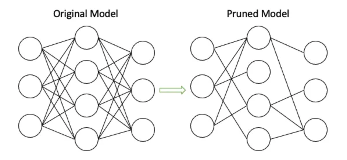
Pruning refers to reducing model parameters by setting certain redundant parameter weights to 0, thereby reducing the model’s parameter count. Structured pruning removes entire neurons or filters, while unstructured pruning removes individual weights (setting weights to zero). Pruning effectively reduces model parameters (by over 90%) while maintaining model accuracy, making it a highly cost-effective compression method for large models.
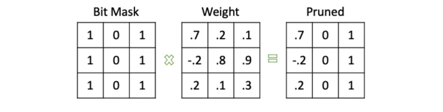
A simple and intuitive pruning method involves setting a threshold; if a weight’s absolute value is below this threshold, it is set to 0. Alternatively, a binary mask of the same size and shape as the weights can represent which parameters need pruning. By multiplying the mask with the weights, we obtain the pruned parameters.
Quantization
Model quantization is a model optimization technique that uses lower-precision data types (like int8) for model parameters (weights) and activations, instead of the 32-bit floating-point format (float32) typically used in training, to reduce computation and memory requirements. Integer data types also speed up matrix multiplications, further enhancing inference speed. There are various quantization methods, such as weight quantization, activation (data) quantization, and gradient quantization.
The two most common quantization types are:
float32 -> float16float32 -> int8
Quantizing from float32 to float16 is straightforward; it merely involves converting model parameters and activation data types from float32 to float16. However, float32 to int8 quantization is more complex, as int8 can only represent integers between -128 and 127, while float32 has a much larger range. Therefore, affine quantization scheme is often used for float32 to int8 quantization.
For a specific float32 parameter range, \([\alpha, \beta]\), we can quantize it to int8 with the following formula:
where \(x\) is the quantized parameter, \(x_q\) is the original parameter, \(S\) is the scaling factor, and \(Z\) is the zero point, representing the int8 value corresponding to 0 in float32. Quantized values \(x_q\) are calculated as follows:
Values outside \([\alpha, \beta]\) in float32 will be clipped to the nearest representable value. Therefore, for any floating-point number \(x\), it can be quantized to int8 using:
🔴 When to use Quantization?
- Dynamic Post-Training Quantization (Dynamic PTQ): loads the trained model for inference and convert model weights ahead of time, and rescale activations on the fly, just before running the computation to determine the scaling factor and zero point. Dynamic PTQ introduces extra overhead during the inference to gain better accuracy and fine-grained scaling for each layer. This is used for situations where the model execution time is dominated by loading weights from memory rather than computing the matrix multiplications — You can parallel compute the scales and doing the weights loading.
- Static Post-Training Quantization (Static PTQ): Load the trained model for inference and convert model weights ahead of time. In order to determine the scaling factor and zero point, it requires a calibration dataset to run through the model. It has no overhead during the inference, but the accuracy is slightly worse than Dynamic PTQ based on the quality of the calibration dataset.
- Quantization-Aware Training (QAT): Training still takes place with full precision, but weights and activations are “fake quantized” during training, which makes the convergence adapt to the quantization. It still requires to do the PTQ after QAT to get the model. But the PTQ process doesn’t require further optimization. QAT has higher quality on the models, but it is expensive to train, especially for large models.
🔴 Quantization in Practical
The simplest way to select the scaling factor is called “MinMax” scaling, which is to find the minimum and maximum value of the weights or activations, and then scale the range to the int8 range. However, this method is not robust enough, especially for the activations, which may have a wide range of values. And MinMax is also very sensitive to outliers.
We use Entropy PTQ + Calibration to achieve better accuracy and robustness. The process is as follows:
- Prepare the calibration dataset, and run the model to get the activations \(P\).
- Select a threshold \(\tau\), and clip the activations \(P\) to get a new distribution \(P'\).
- Conduct the dequantization on \(P'\) to get a distribution \(Q\).
- Calculate the KL divergence between \(P'\) and \(Q\), and use the KL divergence as the loss function to optimize the scaling factor and zero point.
The scaling factor should make we have a minimum KL divergence between the clipped distribution and the quantized distribution. The zero point should make the clipped distribution’s mean as close as possible to the quantized distribution’s mean.
The quantization can be conducted on both weights and activations. So sometimes we choose to use INT8 for weights and INT16 for activations (W8A16). However, W8A16 requires computing the weights and activations in different precision, which may introduce extra quantization/dequantization overhead. So if possible, chosing W8A8 will speedup more (but the accuracy may be worse).
We can also use fine-grained tricks to improve the INT8 activation quantization accuracy:
- Quantize the token/channle level instead of the whole layer. This can improve the accuracy but introduce more quantization operations.
- During the dynamic PTQ, each step we may compute the scales, but in a certain time window, the scales may not change too much. So we can re-use the scale factor for a certain time window to reduce the overhead. For example, re-compute the scale factor every 1000 steps.
For different models, the benefit of quantization may vary. For example, if a language model has small input shapes, the quantization may not bring much benefit. Since it cannot reach the compute bound. So it is better to choose the model with MFU (model flops utilization) larger than 60% to conduct the quantization (can speedup over 30%).
🔴 Selection of the Calibration
Dynamic PTQ are less popular since the speedup is not significant during the inference. And for QAT, since the training of LLM costs a lot, it is not recommended to use QAT for LLMs if it introduces uncertainties in the production environment. So the Static PTQ is the most popular choice for LLMs in production, but it requires a good calibration dataset to get the best accuracy.
- For some application scenarios like recommender system, the model changes frequently (minutes or hours), so the calibration dataset should be updated frequently.
- How to select a dataset with representative samples and diversity is also important, some techniques like active learning can be used (e.g., CoreSet).
- The quantization jobs are inserted into the model swarpping pipeline, led to challenges in the model online serving pipeline.
🔴 FP8 on NVIDIA Hopper
NVIDIA Hopper GPUs (e.g., H100) are supporting FP8 computing, compare to traditional INT8 quantization, it
- Loss of accuracy is less than
INT8quantization.FP8can represent more accurate values thanINT8. - Only need to compute the “tensor-level” scale factor, no need to compute per-token/per-channel scale factor.
- Support dynamic quantization, the accuracy loss is small even without calibration. More friendly to the streaming training/serving pipelines.
Distillation
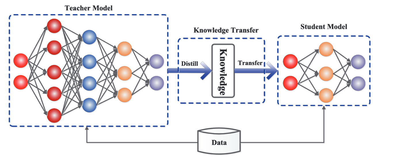
Model distillation trains a smaller model (student model) to approximate a larger model (teacher model), effectively transferring knowledge from the larger model to the smaller one and reducing the smaller model’s parameters. For LLMs, this approach is particularly useful since they contain billions of parameters and are inherently “capable” of various tasks.
One distillation method uses LLMs for labeling unlabeled data on a specific task, which can then train a smaller task-specific model. This method is straightforward but requires substantial unlabeled data and training time. Notably, many GenAI companies (like OpenAI) explicitly prohibit using their models’ generated data to train competitors’ models.
Another popular distillation method is Knowledge Distillation (e.g., DistilBERT), where a smaller model (student) is trained to approximate the output probability distribution of a larger model (teacher). This approach focuses only on the teacher model’s output distribution, not the specific values. However, since it requires the LLM’s full output probability distribution, it can only be performed on open-source LLMs.
Decoding
Decoding speed directly affects LLM inference speed, so several decoding optimization methods exist for LLMs. Traditional LLMs perform inference using autoregressive sampling (as shown below).
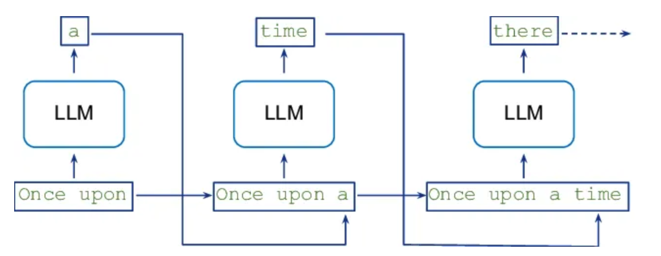
This structure introduces time dependencies in model inference.
Non-autoregressive (NAR) Decoding
The term “Autoregressive” refers to the use of previous time steps to predict the current output. Non-autoregressive decoding generates all outputs simultaneously without depending on prior outputs, effectively removing dependencies between tokens and allowing parallel generation. This method significantly reduces decoding time but may decrease model accuracy.
Speculative Decoding
Speculative Decoding, also known as assisted generation or Medusa, increases LLM inference throughput (~2-3x) with minimal accuracy loss. It requires one or more smaller models to assist LLM inference:
- Target Model: The primary LLM we use
- Small Draft (Approximation) Model: A lighter model primarily for speeding up inference
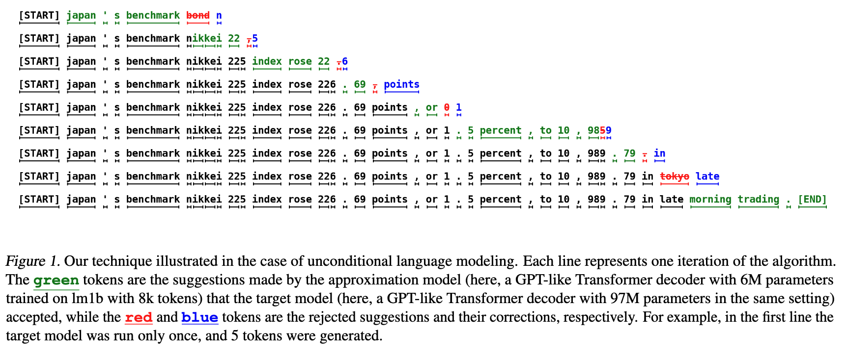
During inference, the Small Draft Model generates a draft output, which the Target Model refines. This approach speeds up inference by generating multiple tokens in a single LLM forward pass. Here is the general workflow (Google DeepMind):
- Step 1: Auto-regressive decode \(K\) tokens from draft model and get final \(p\), append \(K\) new tokens into input \(x\).
- Step 2: Target model forward passes on the \(x\) to get the probability distribution \(q\) of all tokens.
- Step 3: Compare the probability \(q\) and \(p\) to decide whether the token should be kept or rejected. Sample a new token (and its afterward tokens) once rejected.
- Step 4: If all tokens are accepted, sample the next token (based on the token distribution).
- Step 5: loop the process for \(K\) tokens as a pass. The larger \(K\) is the faster inference speedup, the lower latency gain.
Usually, if the target model’s token probability is higher than the draft model’s under a certain tokend, we will accept the token. Like the table shown below:
| Token | I | like | eat | apple | pie | . |
|---|---|---|---|---|---|---|
| Draft Model p(x) | 0.8 | 0.7 | 0.9 | 0.8 | 0.7 | 0.6 |
| Target Model q(x) | 0.9 | 0.8 | 0.8 | 0.3 | 0.8 | 0.4 |
| Accept | Yes | Yes | 8/9 | 3/8 | Yes | 4/6 |
You can see we use the \(\frac{q(x)}{p(x)}\) to decide whether to accept the token or not. If a token is rejected, the rest of the tokens in a total \(K\) will be re-sampled. As you know, based on the above table, the acceptance rate is the key to improve the inference speedup of speculative decoding. If the draft yields tokens that are totally different from the target model, the acceptance rate will be low, and the inference speedup will be limited.
To analyze Speculative Decoding’s performance, suppose the worst case where the draft model’s output is entirely wrong, necessitating corrections by the target model each time. In this case, the inference count will not exceed that of autoregressive decoding. However, if the draft model generates satisfactory values, multiple draft tokens can be validated in a single target model pass, significantly increasing speed.
🔴 Choosing the Right Draft Model
The draft model selection is crucial for speculative decoding. There are few key points to consider:
- Target model is larger than the draft model too much: the rejection rate is high, results in the low efficiency.
- Both models are too small: the performance difference between is not large enough to accelerate the inference.
- The two models are pre-trained with different vocabularies: the candidate distribution is different from the target distribution, the rejection rate is high.
For example, if you are serving LLama3-70b, it is better to use a LLama3-7b as the draft model, rather than another 70b model or other models trained with different vocabularies.
🔴 Spectulative Decoding w/o Draft Models
Since it is so hard to select or train a draft model, many researches are trying to eliminate the draft model. Here are some methods:
- N-gram: Without a new draft model, take a look back of the historical generated distribution vocabulary, pick the top-n for the next draft.
- Medusa: Using extract decoding head for draft generation, without extra model.
- Lookahead: Using Jacobi decoding to guess multiple n-grams in a pass (in parallel using GPU).
- EAGLE: Similar to Medusa, but using a auto-regression head to predict the draft from feature-level instead of token-level. Which is more accurate, results in a higher acceptance rate.
Batching
Batching is a vital optimization method in model inference. By processing multiple input data instances simultaneously, batching maximizes parallel computation, enhancing GPU utilization and increasing inference throughput.
Static Batching
Static batching refers to processing multiple input data instances simultaneously during inference. This approach reduces computation and speeds up inference but requires predefined input sizes. For inputs of different sizes, padding may be necessary.
A simple example is shown below:
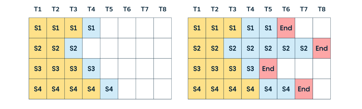
Static batching waits for the “longest” request to finish before returning results. This can lead to extended waiting times for some requests, limiting GPU utilization. Moreover, with a small workload, static batching might cause queuing delays as it waits for enough requests to reach the batch size, further reducing GPU utilization.
Continuous Batching
To address the waiting issue in static batching, continuous batching returns completed requests first, continuing inference for other requests. A visual example is below:
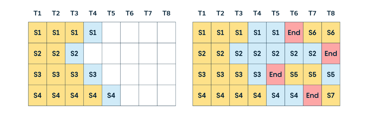
However, a potential issue with this approach is the need to pre-allocate “sufficient” memory space to handle the longest request in each batch to prevent memory overflow. This can lead to memory waste, as the size of incoming requests is unknown in advance. This is why PagedAttention is used to optimize LLM memory management, which we’ll discuss later.
Memory Optimization
The attention mechanism is central to LLMs, enabling them to weigh input data parts differently and focus on relevant information for a task. Improving attention performance enhances inference speed while reducing computation. Since attention is memory-bound, memory management optimization is crucial.
LLM inference memory allocation breakdown:
- Model Parameters: About 65%-70%
- KV Cache: Stores the key and value of the autoregressive model, about 25%-30%
- Others: Activations, intermediate results, about 5%-10%
A simplified version of LLM memory usage during inference:
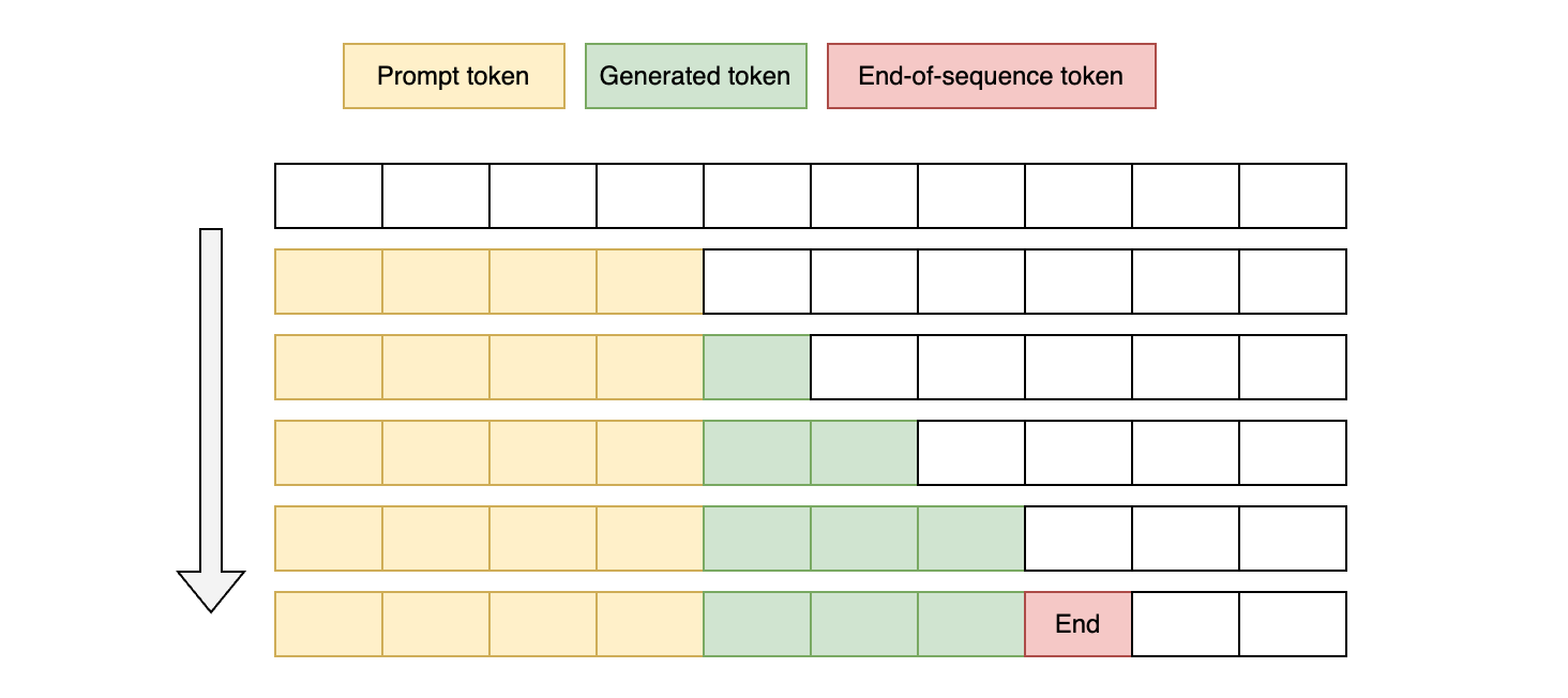
LLM inference consists of two phases:
- Prefill phase: Prompt token preloading and input computation
- Decode phase: Generation of each subsequent token
During the prefill phase, LLM precomputes inputs that remain constant in subsequent generations, leveraging GPU parallelism.
FlashAttention (GPU only)
Regardless of memory type, a general rule is that faster memory is more expensive and has less capacity. FlashAttention uses three types of memory (a sample configuration on an Nvidia A100 + CPU machine):
- CPU main memory (CPU DRAM): Largest capacity, slowest speed (12.8GB/s, >1TB)
- HBM (high bandwidth memory): Fastest speed, moderate capacity (1.5TB/s, 40GB)
- SRAM (on-chip memory): Fastest, smallest capacity (19TB/s, 20MB)
“Graphics memory” typically refers to HBM.
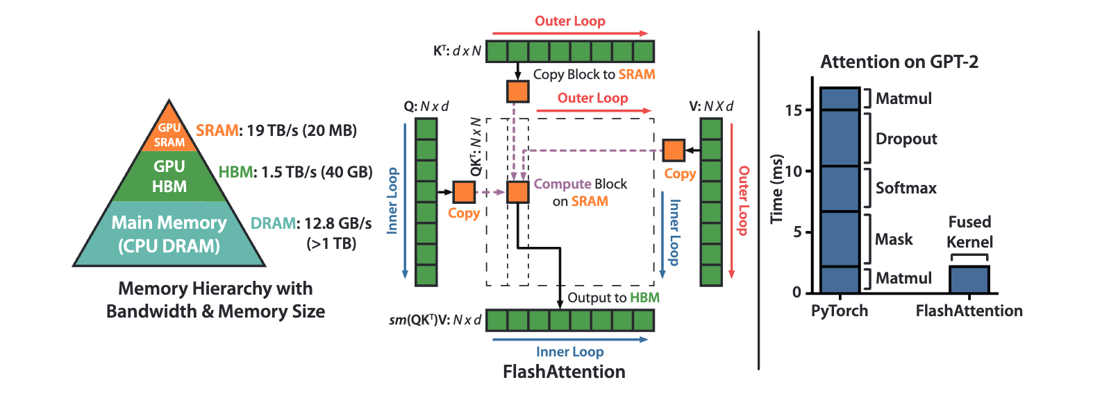
Traditional Transformer inference follows these steps, assuming \(K, V, Q \in R^{N \times d}\) matrices in HBM:
- Load \(Q\) and \(K\) by blocks from HBM, compute \(S = QK^T\) and store \(S\) in HBM.
- Read \(S\) from HBM, compute \(P = \text{softmax}(S)\), and store \(P\) in HBM.
- Load \(P\) from HBM, compute \(O = PV\), and store \(O\) in HBM.
- Return \(O\)
Here, \(K, V, Q\) are key, value, and query matrices, \(S\) is the score matrix, \(P\) is the softmax probability matrix, and \(O\) is the output matrix. The traditional Transformer loads all QKV matrices into HBM for matrix multiplication, which increases HBM read/write operations and reduces inference speed.
The intermediate storage of \(S\) between the first and second steps is unnecessary. If \(S\) is cached in SRAM, HBM read/write operations can be reduced. This approach, known as kernel fusion on GPUs, merges low-level computations to reduce communication overhead. However, SRAM’s limited capacity prevents it from storing the entire \(S\) matrix. FlashAttention addresses this issue with two key ideas:
- Tiling: Used in both forward and backward passes by chunking the NxN softmax/scores matrix into blocks, each small enough for SRAM.
- Recomputation: Used only in the backward pass. This approach stores outputs and softmax normalization statistics to recompute attention matrices, using incremental calculation to obtain precise attention outputs.
PagedAttention
According to our earlier analysis of LLM memory structures, the KV Cache occupies significant memory, making it a primary target for optimization.
PagedAttention, a vLLM optimization inspired by the “virtual memory with paging” concept in traditional OS memory management, divides the KV cache into non-contiguous, fixed-size pages. During inference, only the necessary pages are loaded as needed.
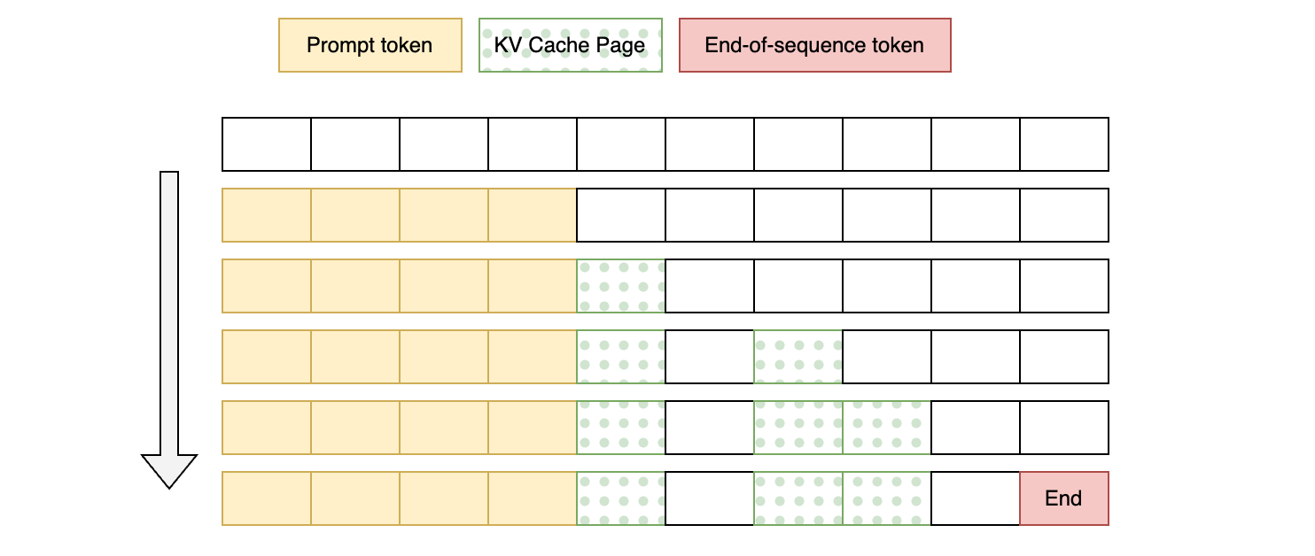
This approach eliminates the need to pre-allocate continuous memory space for the maximum context length and dynamically loads KV cache pages during inference to improve efficiency. However, this method does not guarantee perfect memory utilization; the last block after paging may be partially wasted (vLLM currently achieves less than 4% waste).
Parallelism
Parallel computing is a crucial method for speeding up model inference by dividing the computation into multiple parts for simultaneous execution. Common parallel computing methods include data parallelism, model parallelism, tensor parallelism, and pipeline parallelism. While parallelism is widely used in both model training and inference, Tensor and Pipeline parallelism are more common in inference due to the smaller computation load, more complex data pipeline, and need to handle production uncertainties.
Tensor Parallelism
Tensor parallelism uses multiple GPUs for distributed matrix computation. In LLM inference, tensor operations mainly refer to matrix multiplications of the Key, Value, and Query matrices in the attention mechanism and MLP layers. Matrix multiplications are split across GPUs to utilize multiple devices.
For example, with input vector \(X\), weight matrix \(A\), and output vector \(Y\), we can split the calculation across 3 GPUs as follows:
\[Y = X \cdot A\]is equivalent to
\[\begin{bmatrix} Y_1 \\ Y_2 \\ Y_3 \end{bmatrix} = X \cdot \begin{bmatrix} A_1 & A_2 & A_3 \end{bmatrix}\]where each \(Y_i = X \cdot A_i\) is computed on a separate GPU.
Pipeline Parallelism
Pipeline parallelism involves dividing the model vertically into chunks, each allocated to a different device (stage) for computation. During forwarding, each stage passes intermediate activations to the next stage for parallel computation.
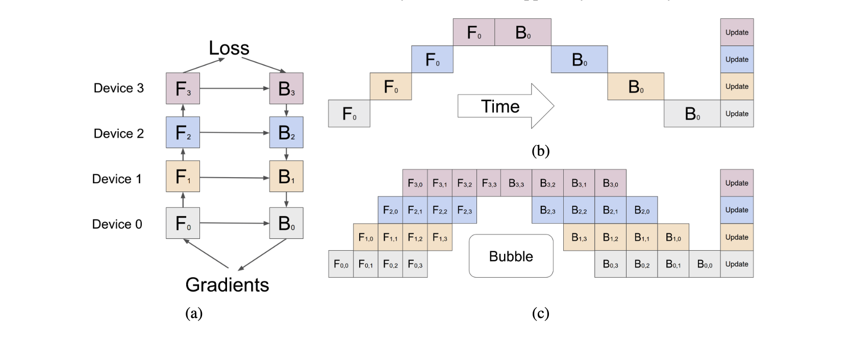
Due to the need for sequential activation transfer and processing across pipeline stages, certain devices idle while awaiting the previous stage’s computation results, reducing pipeline parallelism efficiency, known as “pipeline bubbles.”
Microbatching can reduce pipeline bubbles by dividing input data into smaller batches and interleaving them across stages, reducing waiting times. However, this does not entirely eliminate pipeline bubbles.
Reference
Some of the pictures/links are from the following articles:
- Fast Inference from Transformers via Speculative Decoding
- Model Compression via Pruning
- LLM distillation demystified: a complete guide
- LLM Distillation Explained: Applications, Implementation & More
- FlashAttention: Fast and Memory-Efficient Exact Attention with IO-Awareness
- vLLM: A high-throughput and memory-efficient inference and serving engine for LLMs
- What it means to serve an LLM and which serving technology to choose from
- Mastering LLM Techniques: Inference Optimization
- GPipe: Efficient Training of Giant Neural Networks using Pipeline Parallelism
- Towards Efficient Generative Large Language Model Serving: A Survey from Algorithms to Systems
- PaLM: Scaling Language Modeling with Pathways
- Medusa: Simple LLM Inference Acceleration Framework with Multiple Decoding Heads
- Break the Sequential Dependency of LLM Inference Using Lookahead Decoding
- EAGLE: Speculative Sampling Requires Rethinking Feature Uncertainty
- Quantization-Aware Training for Large Language Models with PyTorch