Lifelong Learning in Modern AI Systems
Table of Contents
What is Lifelong Learning?
Lifelong/Continual learning is often defined as an academic term. In the field of machine learning, it typically refers to continuously training a pre-trained model \(M_{ori}\) on new tasks \({t_1, t_2, ..., t_n}\) while maintaining high accuracy. This learning approach differs from traditional machine learning tasks, which are usually trained on a fixed dataset and tested on another fixed dataset. In such cases, the model’s performance often declines over time or due to changes in the test dataset (data drift).
According to this definition, lifelong learning has two main AI metrics:
- Task Performance: The performance of the model on new tasks, often measured by \(ACC\) (global accuracy) and \(ACC_t\) (accuracy of task \(t\)).
- Catastrophic Forgetting: Whether the model forgets previously learned tasks when learning new ones. This is often measured using \(BWT\) and \(BWT_t\) (the loss in \(ACC\) after learning task \(t\)).
From a systems perspective, additional metrics to consider include:
- Training-Time: The per-epoch average training time for all tasks.
- Extra Parameters: The additional parameters introduced by the lifelong/continual learning strategy.
- Buffer Size: The additional in-memory cache used by the strategy for storing replay data or model weights.
Depending on the type of task, traditional lifelong learning can be further divided into:
- Class-change: A new task adds new classes to the overall task.
- Distribution-change: A new task changes the data of one or more classes, affecting data distribution.
- Task-change: The definition of the task changes with each new learning task.
This is a straightforward and accurate problem definition, but in actual production environments, lifelong learning usually comes with more constraints and requires more engineering implementation details.
Methods of Lifelong Learning
In the past few years, the AI research community has proposed many methods to address the problem of lifelong learning (mainly catastrophic forgetting). These methods can be categorized into three types:
Regularization-based Methods
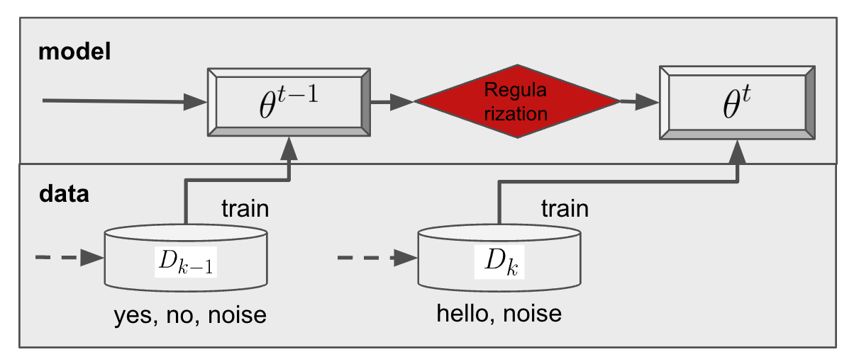
Regularization-based methods involve adding constraints to the loss function to protect pre-trained parameters from being affected by new training tasks. Examples include Elastic Weight Consolidation (EWC), Synaptic Intelligence (SI), and Path Integral (PI).

Specifically, the loss function for such methods is typically formulated as:
\[\mathcal{L}' = \mathcal{L}(F_t(x_t;\theta^t), y_t) + \frac{\lambda}{2} \sum_{i} \Omega^t_i (\theta_i^t - \theta_i^{(t-1)})^2\]where \(\mathcal{L}\) is the loss function for task \(t\), \(\theta^t\) represents the parameters for task \(t\), \(\Omega^t_i\) represents the importance of parameter \(\theta_i^t\), and \(\lambda\) is a hyperparameter. The advantage of this method is that it does not require extra memory for storing data and is computationally efficient. However, it requires information from the previous task’s parameters and tuning the hyperparameter \(\lambda\). The effectiveness of this approach diminishes as the number of tasks increases due to the limited model parameters being unable to accommodate an infinite number of tasks.
Replay-based Methods
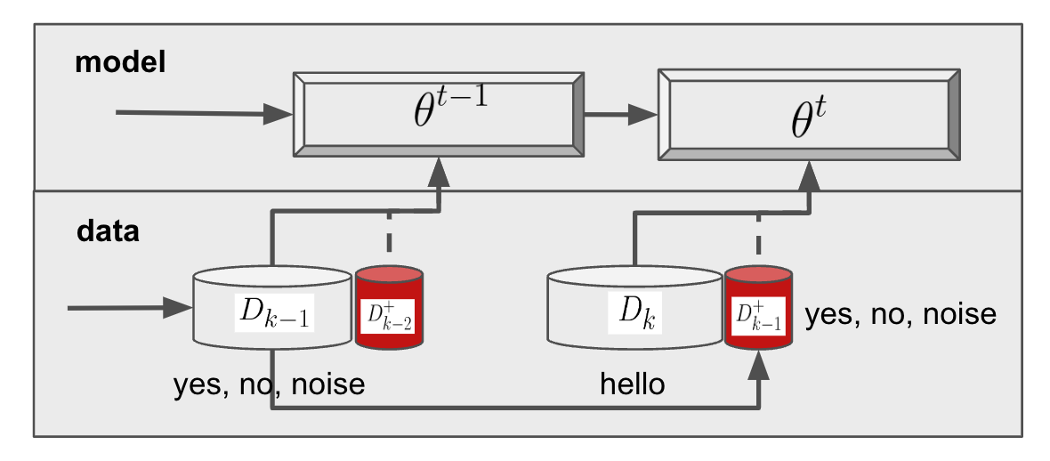
This method avoids catastrophic forgetting by saving historical data or models. Examples include Naive Rehearsal (NR), Gradient Episodic Memory (GEM), and Meta-Experience Replay (MER).

The advantage of this method is that it does not require additional constraints on model parameters. However, it increases memory usage and computational resources as historical data grows with the number of tasks. Selecting high-quality data for the model to “review” is also an important challenge.
Dynamic Expansion Methods
Dynamic expansion methods differ from the previous ones by dynamically increasing the model’s capacity to adapt to new tasks. Examples include Progressive Neural Networks (PNN) and Dynamic Expandable Network (DEN). By dynamically increasing model capacity, the model can better adapt to new tasks while keeping the parameters for old and new tasks separate to reduce catastrophic forgetting.
The advantage of this method is that it handles new tasks effectively but adds more parameters and computational complexity. Lifelong learning is limited by the finite capacity of the model.
Continuous Learning in AI Systems
Frequent paper reading reveals that besides lifelong/continual learning, there is also the concept of continuous learning. What’s the difference between them? Continuous learning is a broader term that not only refers to continually training a model on new tasks but also encompasses many system-level considerations, such as designing a continuous learning system for specific business needs, data pipeline design, model deployment and update strategies, and model monitoring and evaluation strategies.
In such problems, system design becomes crucial. For example, a recommendation system is a typical case of continuous learning. In recommendation systems, user behavior must be continuously learned, and the model updated regularly. The model continuously updates its weights through inference, making its design different from other lifelong learning tasks.
Reinforcement learning is also an example of lifelong learning. In reinforcement learning, the model interacts with the environment and learns new tasks continuously. However, the focus is on designing better strategies, reward functions, and exploration strategies, not on avoiding catastrophic forgetting of past tasks.
Another example is video stream analysis systems (e.g., Ekya NSDI’22, by Romil Bhardwaj et al.). These systems inherently deal with time-series data without a fixed task dataset, requiring continual system updates to maintain high accuracy. Such models often run on edge devices, necessitating efficient cloud-edge collaboration and careful data caching due to limited data storage.
Limited by current model capabilities and evolving business requirements, today’s lifelong learning definitions and solutions still have a long way to go before achieving “AI self-evolution.” However, better system design can maximize the benefits of lifelong learning. The general process includes:
Better Monitoring
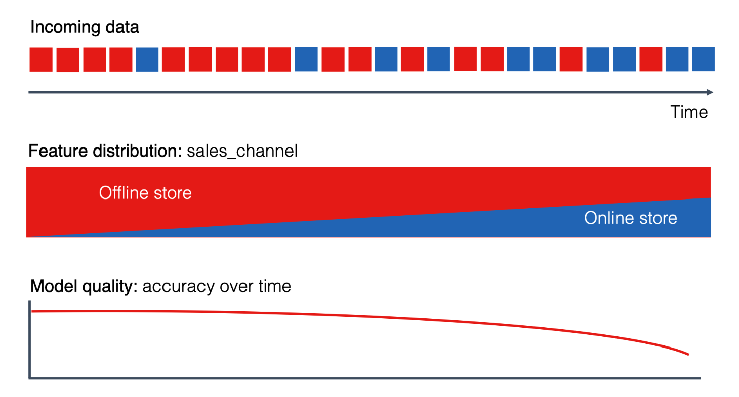
To handle a continuously changing deployment environment, the system must first collect and analyze data to detect changes in both data and models. A drop in model performance due to data distribution changes should trigger model fine-tuning or retraining.

Main drift detection methods include:
- Data Distribution Comparison: Regularly comparing new and old data distributions to detect changes.
- Model Performance Monitoring: Regularly checking model performance and triggering fine-tuning or retraining if performance drops.
Better Model Deployment
To adapt to a changing deployment environment, the system must be able to quickly deploy new models and roll back to previous versions when needed. This requires a hot-swapping system that does not disrupt online services. Conduct A/B testing beforehand to ensure the new model’s performance and safety.
In large-scale distributed systems, you can deploy a new model on a subset of nodes and gradually expand, minimizing risks if the deployment fails. Node selection, model gray release, and rollback strategies depend on specific business needs.
Learning on Edge Devices?
Learning on edge devices is a good approach for preserving user data privacy while providing “personalized” services. However, it is limited by:
- Storage space: Edge devices have limited storage, so they cannot store large amounts of historical data or model parameters.
- Computational resources: Edge devices have limited computing power, making large-scale model training infeasible and requiring fast model updates.
A common solution is to design an efficient cloud-edge collaboration system. The cloud handles the base pre-trained model updates (usually monthly), while the edge device performs frequent model updates (daily). The edge device also needs an efficient data caching system to ensure sufficient training data without consuming excessive storage.
Large-scale?
As model size (parameter count) increases, the cost of continuous learning rises, making it more challenging. Generally, larger models are better at generalizing to similar tasks, but they require more computation, data, and time to learn new tasks.
For large language models (LLMs), training involves more than simple data input and parameter updates—it is a comprehensive pipeline, including data preprocessing, pretraining, and post-training with Reinforcement Learning from Human Feedback (RLHF) and Alignment with Human Values (AHV). This makes retraining large models costly, and even fine-tuning requires significant resources. While leveraging LLMs’ in-context learning, prompt engineering, or using RAG can make models “adapt” to new tasks, updating the model’s structure and reducing system learning costs remain unsolved challenges.
One direct approach is to use the understanding and code-generation capabilities of LLMs to explore completing traditional ML tasks end-to-end. If feasible, small models generated from this approach could perform RAG or fine-tuning to reduce the cost of continuous learning. The next step would involve generative model updates using LLM-generated code to achieve true continuous learning.