<?xml version="1.0" encoding="utf-8"?><feed xmlns="http://www.w3.org/2005/Atom" ><generator uri="https://jekyllrb.com/" version="3.10.0">Jekyll</generator><link href="https://blog.huangyz.name//feed.xml" rel="self" type="application/atom+xml" /><link href="https://blog.huangyz.name//" rel="alternate" type="text/html" /><updated>2026-02-16T06:42:34+00:00</updated><id>https://blog.huangyz.name//feed.xml</id><title type="html">Yizheng’s Blog</title><subtitle>Generative AI, Large-scale ML, Distributed Systems, and more.</subtitle><author><name>Yizheng Huang</name></author><entry><title type="html">2025: 纯粹, 烂漫, 少年心气</title><link href="https://blog.huangyz.name//life/2025/12/26/notes.html" rel="alternate" type="text/html" title="2025: 纯粹, 烂漫, 少年心气" /><published>2025-12-26T00:00:00+00:00</published><updated>2025-12-26T00:00:00+00:00</updated><id>https://blog.huangyz.name//life/2025/12/26/notes</id><content type="html" xml:base="https://blog.huangyz.name//life/2025/12/26/notes.html"><![CDATA[<p>杨绛说：“我们曾如此渴望命运的波澜，到最后才发现，人生最曼妙的风景，竟是内心的淡定和从容”。</p>

<p>2015-2025，希望眼前的自己不论经历了多少仍然拥有对这个世界纯粹的好奇，依然烂漫而真诚面对周围的人和事，在享受自由的同时追求内心的平静和坚定。</p>

<p>感恩。</p>]]></content><author><name>Yizheng</name></author><category term="life" /><summary type="html"><![CDATA[杨绛说：“我们曾如此渴望命运的波澜，到最后才发现，人生最曼妙的风景，竟是内心的淡定和从容”。]]></summary></entry><entry><title type="html">A Close-look at RAG System Optimization</title><link href="https://blog.huangyz.name//tech/2024/10/18/notes.html" rel="alternate" type="text/html" title="A Close-look at RAG System Optimization" /><published>2024-10-18T00:00:00+00:00</published><updated>2024-10-18T00:00:00+00:00</updated><id>https://blog.huangyz.name//tech/2024/10/18/notes</id><content type="html" xml:base="https://blog.huangyz.name//tech/2024/10/18/notes.html"><![CDATA[<h3 id="table-of-contents">Table of Contents</h3>

<ul>
  <li><a href="#an-introduction-to-rag">An Introduction to RAG</a></li>
  <li><a href="#vector-database">Vector Database</a></li>
  <li><a href="#chunking">Chunking</a>
    <ul>
      <li><a href="#dynamic-chunk-size">Dynamic Chunk Size</a></li>
      <li><a href="#chunk-overlap">Chunk Overlap</a></li>
      <li><a href="#context-enrichment">Context Enrichment</a></li>
    </ul>
  </li>
  <li><a href="#re-ranking">Re-ranking</a>
    <ul>
      <li><a href="#agent-based-re-ranking">Agent-based Re-ranking</a></li>
      <li><a href="#graph-based-re-ranking">Graph-based Re-ranking</a></li>
      <li><a href="#hypothetical-questionshyde">Hypothetical Questions/HyDE</a></li>
      <li><a href="#fusion-retrieval">Fusion Retrieval</a></li>
    </ul>
  </li>
  <li><a href="#query-transformation">Query Transformation</a>
    <ul>
      <li><a href="#multi-step-query-transformations">Multi-Step Query Transformations</a></li>
      <li><a href="#query-rewriting">Query Rewriting</a></li>
      <li><a href="#query-expansion">Query Expansion</a></li>
      <li><a href="#query-routing">Query Routing</a></li>
    </ul>
  </li>
</ul>

<h3 id="an-introduction-to-rag">An Introduction to RAG</h3>

<p>RAG (Retrieval-Augmented Generation) is a new paradigm in building large language models (LLM) agents. It improves the accuracy and reliability of generative AI applications by leveraging the facts fetched from external sources.</p>

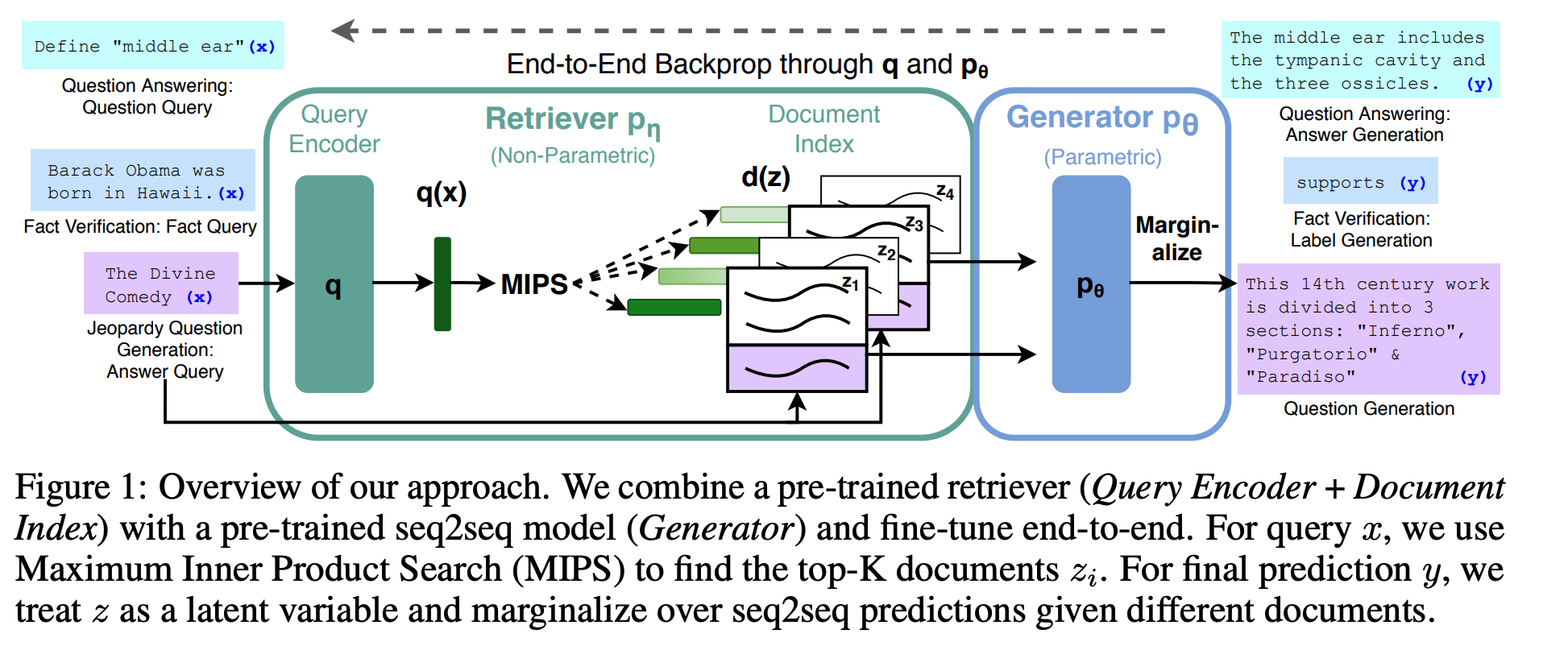
<p>The concept of the RAG model was proposed in the paper <strong>Retrieval-Augmented Generation for Knowledge-Intensive NLP Tasks</strong> <a href="https://arxiv.org/abs/2005.11401">(2020, Patrick Lewis et al)</a>, which combines the strengths of parametric and non-parametric memory. The RAG model is composed of two components: a retriever and a generator, and the whole pipeline is trained end-to-end.</p>

<p><img src="https://s2.loli.net/2024/11/29/dCT8WsuwkYQZL1f.png" alt="" /></p>

<p>The retriever is responsible for fetching relevant facts from external sources, while the generator is responsible for generating text based on the retrieved facts. The paper was published before the release of ChatGPT, and due to the in-context learning ability of LLMs, there is no need to train the RAG model for LLM end-to-end. The information retrieved by the retriever can be directly fed into the generator to generate the text. (During the LLM fine-tuning stage, the RAG model can be tuned end-to-end to enhance performance).</p>

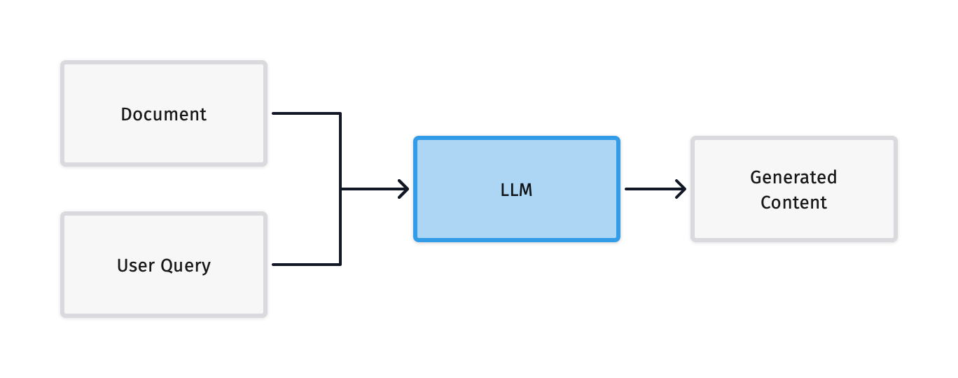
<p>Using the in-context learning capability of LLMs, we can design a simple RAG system as shown below:</p>

<p><img src="https://s2.loli.net/2024/11/29/V8AnraX6vHK3pif.png" alt="" /></p>

<p>This system simply combines external information with the user query and inputs it into the LLM to generate a more accurate response. However, this system also has some obvious drawbacks:</p>

<ul>
  <li><strong>Unable to handle large amounts of external information:</strong> Due to the context window length limitations of Transformer models, inputting a large amount of information can lead to memory issues and information redundancy.</li>
  <li><strong>Unable to filter information based on the user query:</strong> Since the information is directly input into the LLM, it cannot specifically retrieve relevant information based on the user query, leading to potentially inaccurate responses.</li>
</ul>

<p>Next, we will introduce how to optimize the RAG model to address the above issues.</p>

<h3 id="vector-database">Vector Database</h3>

<p>In practical applications of the RAG model, we often need to use a vector database to store external information. This vector database can be a simple key-value database or a more complex graph database.</p>

<p>Let’s take the <code class="language-plaintext highlighter-rouge">upsert</code> API of <a href="https://www.trychroma.com/">ChromaDB</a> as an example:</p>

<div class="language-python highlighter-rouge"><div class="highlight"><pre class="highlight"><code><span class="n">collection</span><span class="p">.</span><span class="n">upsert</span><span class="p">(</span>
    <span class="n">documents</span><span class="o">=</span><span class="p">[</span>
        <span class="s">"This is a document about pineapple"</span><span class="p">,</span>
        <span class="s">"This is a document about oranges"</span>
    <span class="p">],</span>
    <span class="n">ids</span><span class="o">=</span><span class="p">[</span><span class="s">"id1"</span><span class="p">,</span> <span class="s">"id2"</span><span class="p">]</span>
<span class="p">)</span>
</code></pre></div></div>

<p>Here, <code class="language-plaintext highlighter-rouge">documents</code> is a list containing two documents, and <code class="language-plaintext highlighter-rouge">ids</code> are the IDs of these two documents.</p>

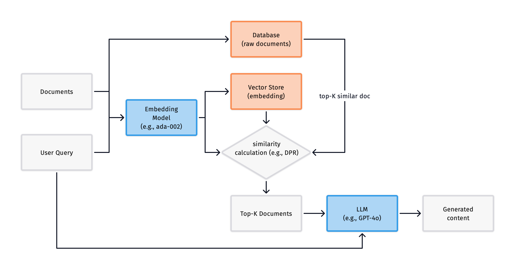
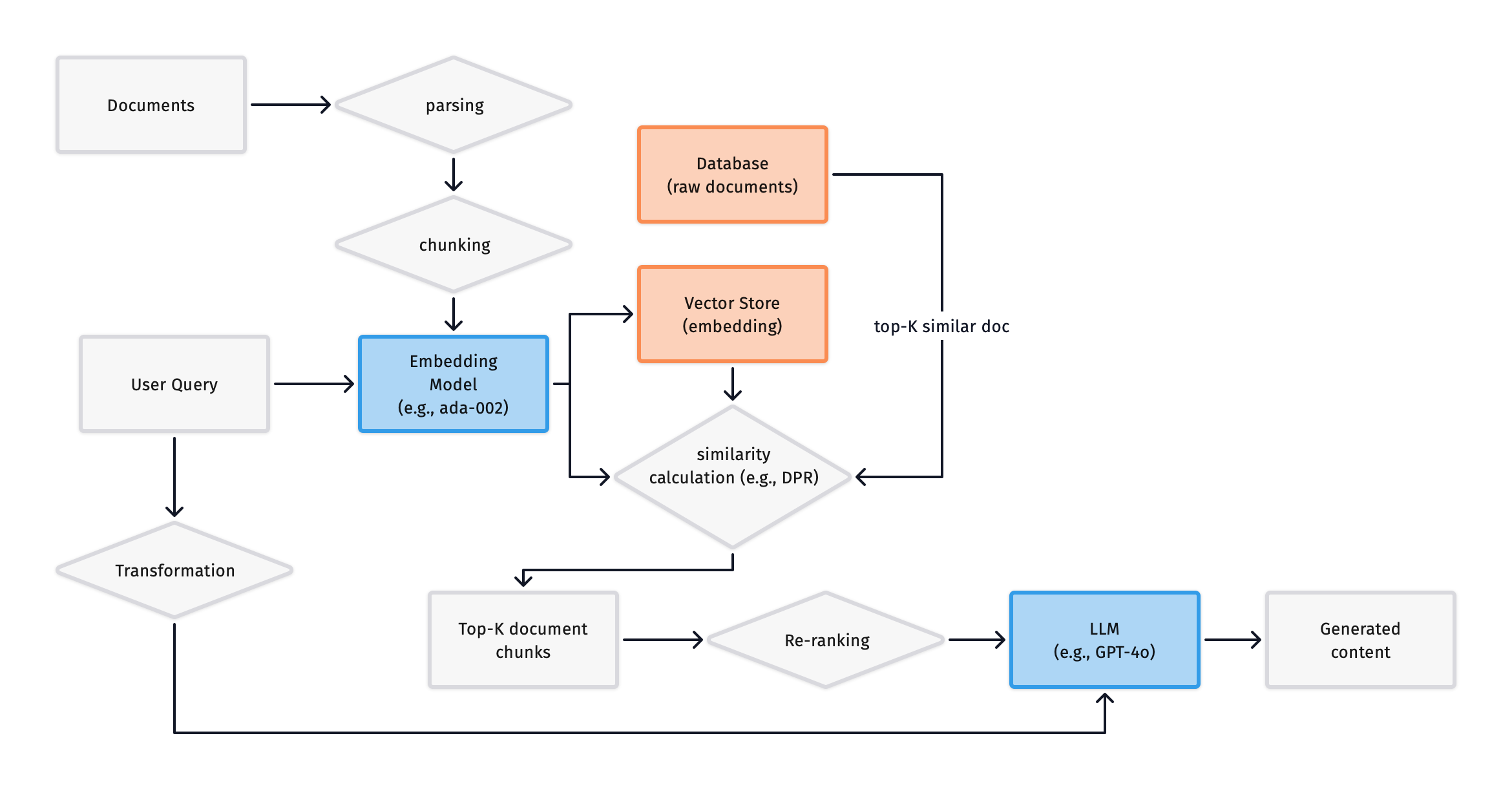
<p>Based on such an API, we can also design and add a simple vector database to the above RAG pipeline, as shown below:</p>

<p><img src="https://s2.loli.net/2024/11/29/wWs8VfI9CrUkd7D.png" alt="" /></p>

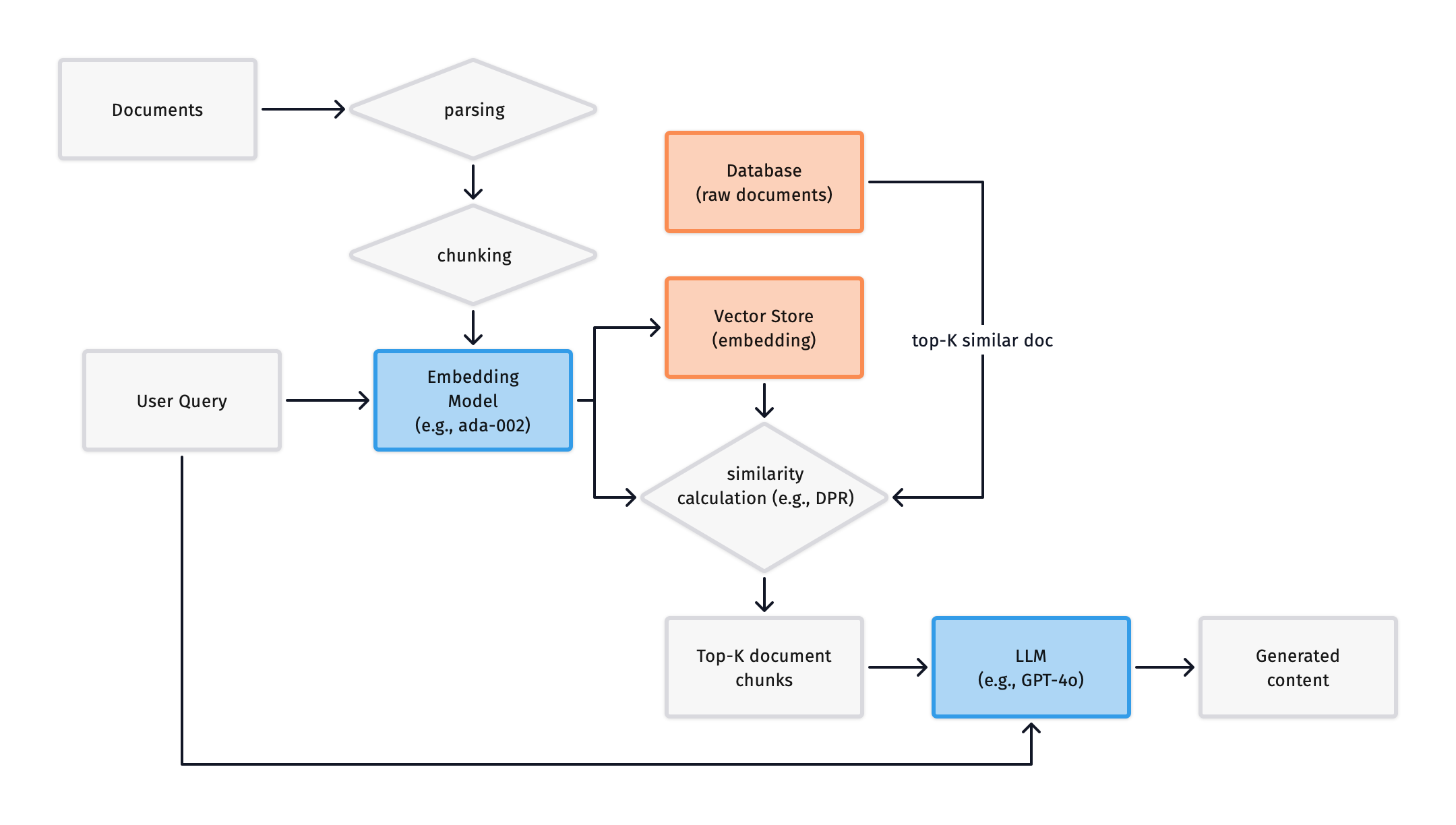
<p>In this system, the original document data is stored in the <code class="language-plaintext highlighter-rouge">Database</code>, while the corresponding embeddings are stored in the <code class="language-plaintext highlighter-rouge">Vector Store</code>. Documents are converted into embeddings by the <code class="language-plaintext highlighter-rouge">Embedding Model</code> and stored in advance. When a query is made, the query is converted into an embedding by the <code class="language-plaintext highlighter-rouge">Embedding Model</code> and compared with all embeddings in the <code class="language-plaintext highlighter-rouge">Vector Store</code> to calculate similarity (<a href="https://arxiv.org/abs/2004.04906">Vladimir Karpukhin et al, 2020</a>), returning the most similar documents.</p>

<p>Additionally, a <code class="language-plaintext highlighter-rouge">Vector Index</code> between the <code class="language-plaintext highlighter-rouge">Database</code> and <code class="language-plaintext highlighter-rouge">Vector Store</code> contains the mapping between document IDs and embeddings. For large-scale text retrieval, we can use libraries like <a href="https://faiss.ai/">FAISS</a>, <a href="https://github.com/nmslib/nmslib">nmslib</a>, or <a href="https://github.com/spotify/annoy">Annoy</a>.</p>

<p>In summary, the introduction of a vector database solves the second issue mentioned above: the system can specifically search for information based on the user query. However, when dealing with an excessive amount of text, it is unreasonable to input an overly long text as a single vector into the LLM, so further optimization of the system is needed.</p>

<h3 id="chunking">Chunking</h3>

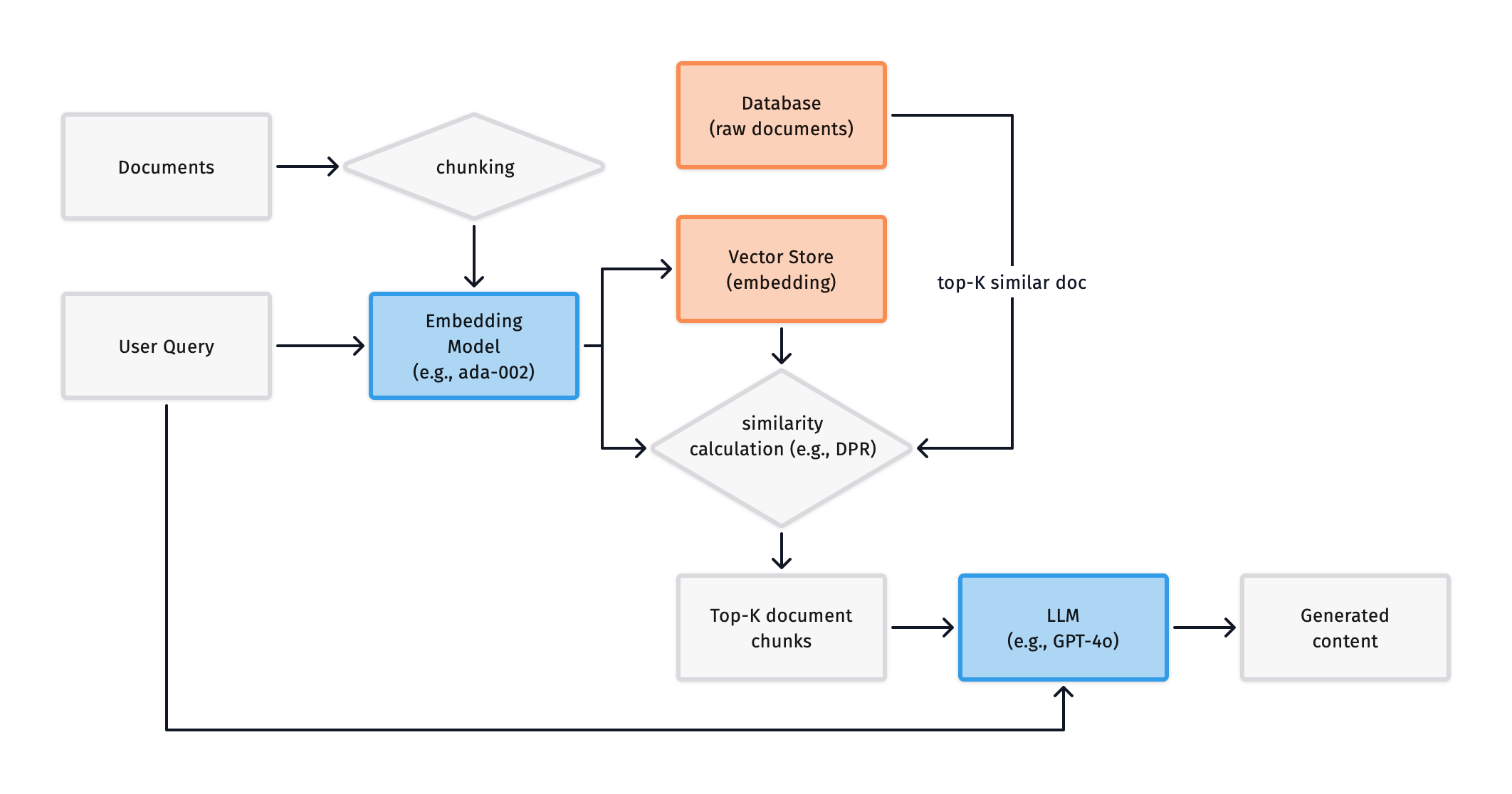
<p>To solve the problem of long input text, we can split the text into chunks and store each chunk separately in the vector database, as shown below:</p>

<p><img src="https://s2.loli.net/2024/11/29/JGV7UgxeI3mpMdK.png" alt="" /></p>

<p>We process the document by splitting it into chunks before inputting it, solving the problem of excessive input length. However, this design also introduces a new issue: the relationships between chunks may be lost, leading to inaccurate responses. For example, if an article is split into two chunks, during response generation, we might generate two unrelated responses—because splitting chunks too crudely may separate a complete sentence into two “incoherent” segments, leading to LLM hallucinations.</p>

<p>The choice of chunk size becomes crucial in this context. On the one hand, we want the chunk size to be as large as possible to minimize loss of relationships between chunks; on the other hand, we want the chunk size to be as small as possible to reduce system load and adapt to models with context window limitations.</p>

<h4 id="dynamic-chunk-size">Dynamic Chunk Size</h4>

<p>This is a more flexible chunking approach where we dynamically adjust the chunk size based on semantics. For example, if we need to split a code file, we should dynamically adjust the chunk size based on the semantics of the code, such as treating a function as a chunk or an if-else statement as a chunk. These chunks may have different sizes, so we need to design a <code class="language-plaintext highlighter-rouge">max_chunk_size</code> to ensure system stability.</p>

<p>For text data, paragraph-based chunking can be adopted, treating each paragraph (or chapter) as a chunk. Under stable system conditions, we can set a relatively large chunk size.</p>

<p>Thus, we can add a <code class="language-plaintext highlighter-rouge">parsing</code> module to the system to preprocess the text (semantically segment it) before chunking, as shown below:</p>

<p><img src="https://s2.loli.net/2024/11/29/uM4x75QthCL1eWj.png" alt="" /></p>

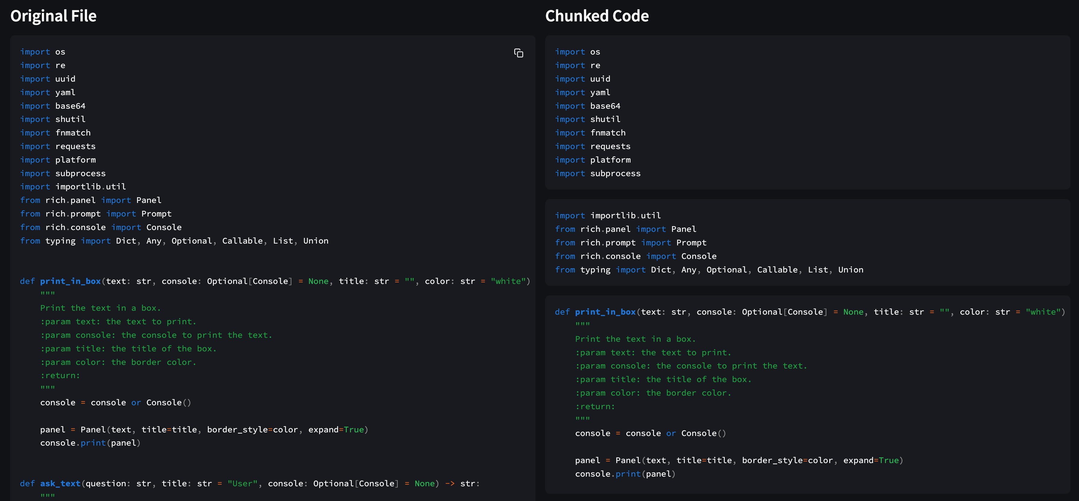
<p>The above code RAG system, after processing by the parser, can obtain semantically related chunks, as shown:</p>

<p><img src="https://s2.loli.net/2024/11/29/xr1CDkj5NHKiYnu.png" alt="" /></p>

<h4 id="chunk-overlap">Chunk Overlap</h4>

<p>To address the problem of loss of relationships between chunks, we can introduce the concept of <strong>chunk overlap</strong>, where there is some overlap of information between chunks. As shown:</p>

<p><img src="https://s2.loli.net/2024/11/29/uZnoMcFev2ijXgL.png" alt="" /></p>

<p>The downside of this approach is that more chunks are needed to store the same amount of document, resulting in additional storage overhead.</p>

<h4 id="context-enrichment">Context Enrichment</h4>

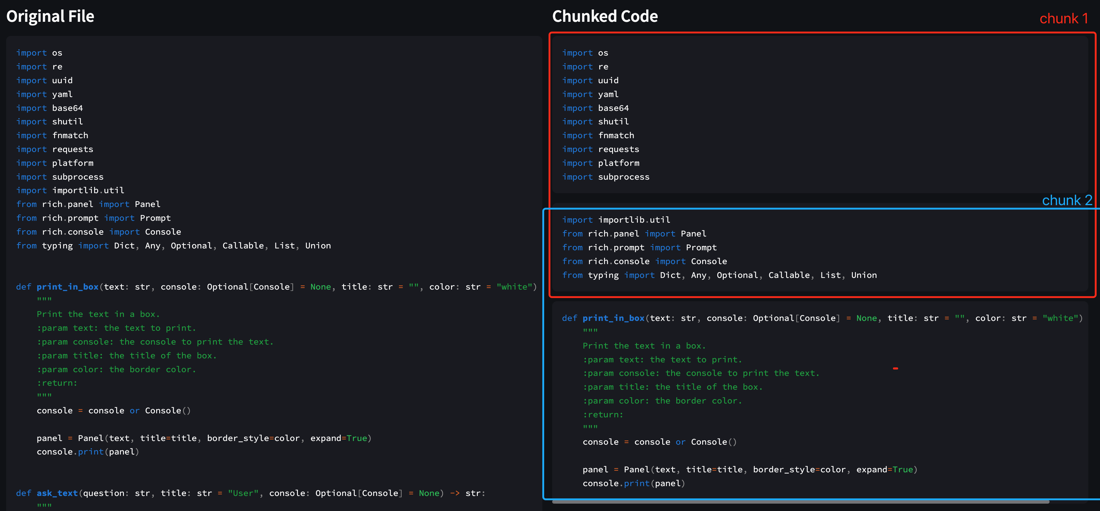
<p>The loss of information between chunks can also be addressed through <strong>context enrichment</strong>. During response generation, we can expand the existing chunk to include more relevant information within the context window without compromising retrieval efficiency. For example, when constructing a code RAG system, we can perform dynamic chunking of code to retain semantic information, but each chunk may vary in size. This is suboptimal for data storage, but through context enrichment, we can expand all chunks to <code class="language-plaintext highlighter-rouge">max_chunk_size</code>, ensuring that all chunks have a uniform size while introducing chunk overlaps.</p>

<p>Taking the Code RAG example mentioned earlier:</p>

<p><img src="https://s2.loli.net/2024/11/29/GLKNrVE9hQa5fis.png" alt="" /></p>

<p>We enriched the context of chunks to ensure no loss of information between code blocks while maintaining consistent chunk sizes (red and blue boxes).</p>

<h3 id="re-ranking">Re-ranking</h3>

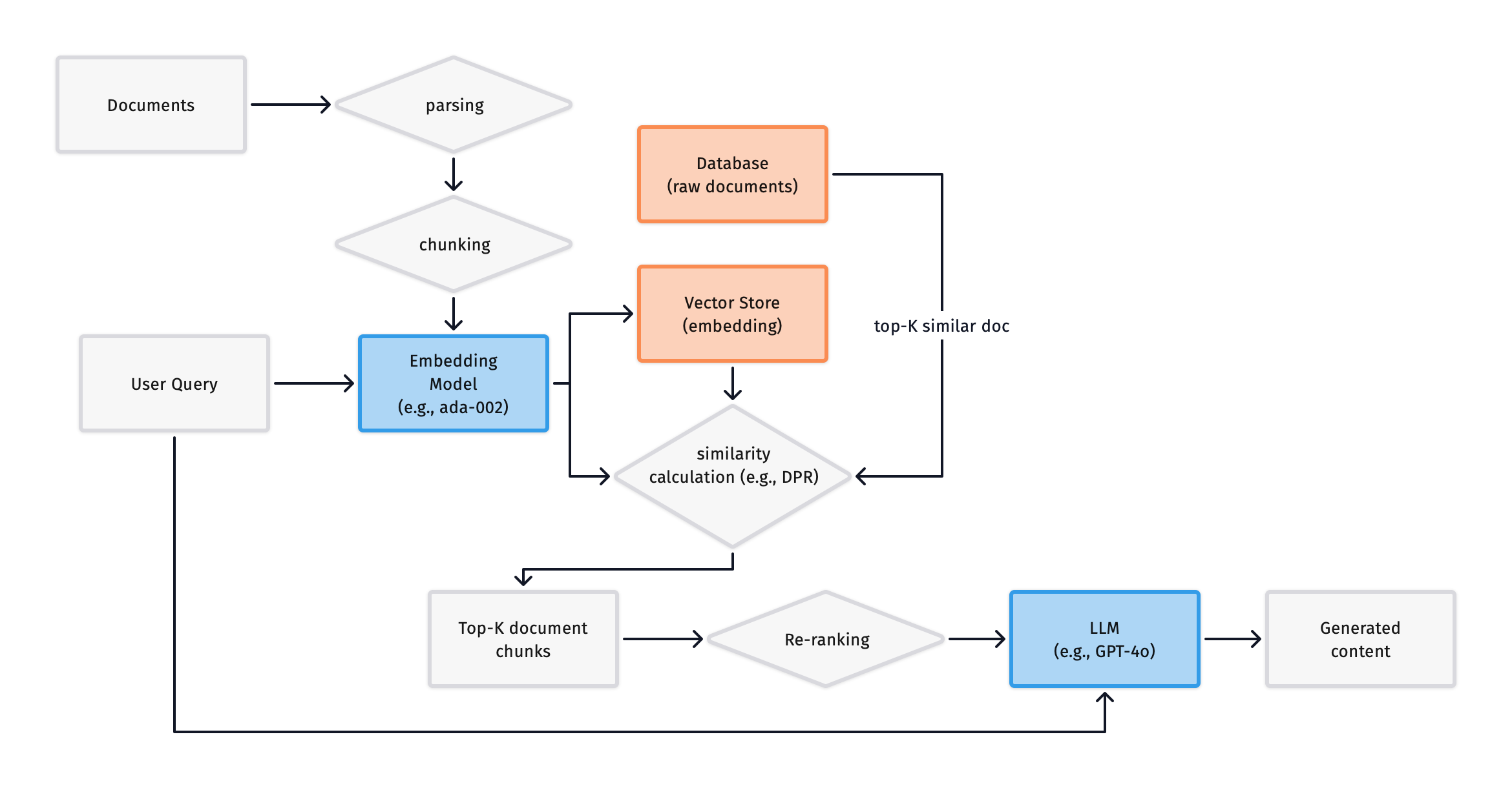
<p>We call it Re-ranking because we introduce a new <code class="language-plaintext highlighter-rouge">Ranker</code> module here, whose purpose is to re-order the results returned by the <code class="language-plaintext highlighter-rouge">Retriever</code> to ensure that the most relevant information is input into the LLM. As shown below:</p>

<p><img src="https://s2.loli.net/2024/11/29/QicmvuYaKBZRsEO.png" alt="" /></p>

<p>The principle is straightforward: since the retriever in a RAG model matches based on vector similarity, the match may be “most relevant” but not necessarily “most useful”. So how do we re-order it?</p>

<h4 id="agent-based-re-ranking">Agent-based Re-ranking</h4>

<p>We can use another model for ranking. This model could be a smaller one or an LLM-based agent. Its task is to determine which documents are most useful and then input those into the LLM. This design ensures that the most useful information is input into the LLM but also introduces additional complexity, as we need an extra model for ranking.</p>

<h4 id="graph-based-re-ranking">Graph-based Re-ranking</h4>

<p>We can use a graph model for ranking. A knowledge graph can compute the intrinsic relationships between chunks, extract entities, and understand the text from a high-level perspective. For some high-level tasks (e.g., summarization), graph-based re-ranking is an excellent choice.</p>

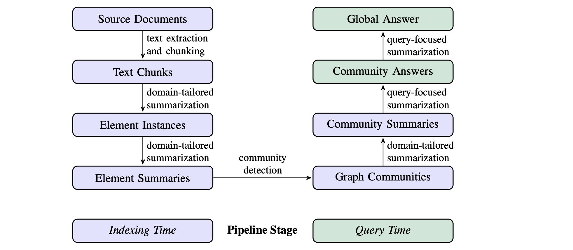
<p><a href="https://arxiv.org/abs/2404.16130">GraphRAG (Darren Edge et al, 2024)</a> proposed enhancing RAG using graphs, as shown below:</p>

<p><img src="https://s2.loli.net/2024/11/29/oNdKwRthbafQljv.png" alt="" /></p>

<p>For retrieved text chunks:</p>

<ul>
  <li>Construct a graph: Model the entities and relationships in the text into a knowledge graph.</li>
  <li>Community detection and summary generation: Use community detection algorithms (e.g., Leiden) to partition the graph into a set of closely related entity communities. LLM then generates summaries for these communities, providing a descriptive summary for each community.</li>
  <li>Query processing and final answer generation: For the user query, each community’s summary is used to generate part of the response, and these parts are then summarized into a final answer.</li>
</ul>

<p>This method supports answering global awareness questions for datasets and large-scale texts, especially when the data scale exceeds millions of tokens.</p>

<h4 id="hypothetical-questionshyde">Hypothetical Questions/HyDE</h4>

<p>To better match the retrieved chunks with the user’s query, we can generate “questions” for each chunk. This design is intuitive because, in <code class="language-plaintext highlighter-rouge">question-answer</code> paired datasets, matching the question with the user’s query is more in line with human thought processes. We then rank the chunks based on question similarity to ensure that “useful” data is given higher priority. HyDE works in the opposite way—it generates hypothetical answers for each query and then ranks the chunks based on the similarity between these answers and the chunks. We can view HyDE as a method for query transformation (which we will introduce shortly).</p>

<h4 id="fusion-retrieval">Fusion Retrieval</h4>

<p>This is another common re-ranking method. We can use both embedding similarity calculation and keyword-based search methods (e.g., <a href="https://en.wikipedia.org/wiki/Okapi_BM25">BM25</a>) to rank results. The results of both methods are fused to enhance retrieval effectiveness.</p>

<h3 id="query-transformation">Query Transformation</h3>

<p>Apart from post-processing, we can also process the query beforehand to ensure more accurate information retrieval. As shown below:</p>

<p><img src="https://s2.loli.net/2024/11/29/C4iyD9TQoXN37Aa.png" alt="" /></p>

<p>We added a <code class="language-plaintext highlighter-rouge">Transformation</code> module, and now let’s discuss some specific methods:</p>

<h4 id="multi-step-query-transformations">Multi-Step Query Transformations</h4>

<p>The multi-step query transformation approach splits the user’s query into sequential subquestions. This method can be handy when working with complex questions. For example, if the user asks a question like “Are there any good restaurants near me?”, the system can split the question into two subquestions:</p>

<ul>
  <li>“What are the good restaurants?”</li>
  <li>“Are there any restaurants near me?”.</li>
</ul>

<p>The information retrieved from the database can then be used to answer these subquestions, and the final answer can be generated by combining the results.</p>

<h4 id="query-rewriting">Query Rewriting</h4>

<p>Query rewriting is another method that can be used to improve the accuracy of information retrieval. In this approach, the system rewrites the user’s query to make it more specific or relevant to the information stored in the database. For example, if the user asks a question like “What are the best pizza places in New York?”, the system can rewrite the query to “What are the best Italian restaurants in New York?” to make it more specific. This can help the system retrieve more accurate information from the database.</p>

<h4 id="query-expansion">Query Expansion</h4>

<p>By expanding the query, we can broaden the match for retrieval information. The principle is to expand the query using synonyms or similar words to increase the amount of information retrieved. The advantage of this method is its simplicity, but it also has some drawbacks: the expanded query may introduce noise, leading to inaccurate retrieval.</p>

<p>An example question of query expansion: “What is the most colorful bird in the world?” can be expanded to “What is the most colorful bird in the world? (e.g., parrot, peacock)”, where some examples of colorful birds are provided.</p>

<h4 id="query-routing">Query Routing</h4>

<p>This is suitable for complex scenarios involving multiple databases. We need to route the query to the appropriate database for retrieval. One example is multimodal RAG, where we need to send image queries to an image database and text queries to a text database, then fuse the retrieval results before inputting them into the LLM. Image data requires additional models to compute embeddings, which are then matched with text data.</p>]]></content><author><name>Yizheng Huang</name></author><category term="tech" /><summary type="html"><![CDATA[Table of Contents]]></summary></entry><entry><title type="html">Serving LLMs in Production - The Optimization</title><link href="https://blog.huangyz.name//tech/2024/08/12/notes.html" rel="alternate" type="text/html" title="Serving LLMs in Production - The Optimization" /><published>2024-08-12T00:00:00+00:00</published><updated>2024-08-12T00:00:00+00:00</updated><id>https://blog.huangyz.name//tech/2024/08/12/notes</id><content type="html" xml:base="https://blog.huangyz.name//tech/2024/08/12/notes.html"><![CDATA[<h3 id="table-of-contents">Table of Contents</h3>

<ul>
  <li><a href="#post-training-model-compression">Post-training Model Compression</a>
    <ul>
      <li><a href="#pruning">Pruning</a></li>
      <li><a href="#quantization">Quantization</a></li>
      <li><a href="#distillation">Distillation</a></li>
    </ul>
  </li>
  <li><a href="#decoding">Decoding</a>
    <ul>
      <li><a href="#non-autoregressive-nar-decoding">Non-autoregressive (NAR) Decoding</a></li>
      <li><a href="#speculative-decoding">Speculative Decoding</a></li>
    </ul>
  </li>
  <li><a href="#batching">Batching</a>
    <ul>
      <li><a href="#static-batching">Static Batching</a></li>
      <li><a href="#continuous-batching">Continuous Batching</a></li>
    </ul>
  </li>
  <li><a href="#memory-optimization">Memory Optimization</a>
    <ul>
      <li><a href="#flashattention-gpu-only">FlashAttention (GPU only)</a></li>
      <li><a href="#pagedattention">PagedAttention</a></li>
    </ul>
  </li>
  <li><a href="#parallelism">Parallelism</a>
    <ul>
      <li><a href="#tensor-parallelism">Tensor Parallelism</a></li>
      <li><a href="#pipeline-parallelism">Pipeline Parallelism</a></li>
    </ul>
  </li>
  <li><a href="#reference">Reference</a></li>
</ul>

<hr />

<h3 id="post-training-model-compression">Post-training Model Compression</h3>

<p>Common post-training model compression methods include pruning, quantization, and distillation. These methods effectively reduce model parameters, increase inference speed, and largely maintain model accuracy.</p>

<h4 id="pruning">Pruning</h4>

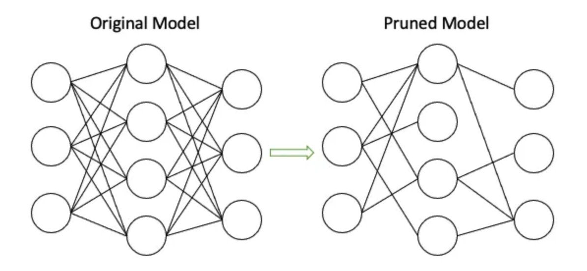
<p><img src="https://s2.loli.net/2024/11/07/reHXxJkUgLVAp2m.png" alt="Pruning" /></p>

<p>Pruning refers to reducing model parameters by setting certain redundant parameter weights to 0, thereby reducing the model’s parameter count. Structured pruning removes entire neurons or filters, while unstructured pruning removes individual weights (setting weights to zero). Pruning effectively reduces model parameters (by over 90%) while maintaining model accuracy, making it a highly cost-effective compression method for large models.</p>

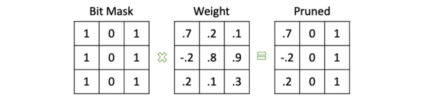
<p>A simple and intuitive pruning method involves setting a threshold; if a weight’s absolute value is below this threshold, it is set to 0. Alternatively, a binary mask of the same size and shape as the weights can represent which parameters need pruning. By multiplying the mask with the weights, we obtain the pruned parameters.</p>

<p><img src="https://s2.loli.net/2024/11/07/CGmwNJL9Z4YpDFc.png" alt="Bit Mask" /></p>

<h4 id="quantization">Quantization</h4>

<p>Model quantization is a model optimization technique that uses lower-precision data types (like int8) for model parameters (weights) and activations, instead of the 32-bit floating-point format (float32) typically used in training, to reduce computation and memory requirements. Integer data types also speed up matrix multiplications, further enhancing inference speed. There are various quantization methods, such as weight quantization, activation (data) quantization, and gradient quantization.</p>

<p>The two most common quantization types are:</p>

<ul>
  <li><code class="language-plaintext highlighter-rouge">float32 -&gt; float16</code></li>
  <li><code class="language-plaintext highlighter-rouge">float32 -&gt; int8</code></li>
</ul>

<p>Quantizing from <code class="language-plaintext highlighter-rouge">float32</code> to <code class="language-plaintext highlighter-rouge">float16</code> is straightforward; it merely involves converting model parameters and activation data types from <code class="language-plaintext highlighter-rouge">float32</code> to <code class="language-plaintext highlighter-rouge">float16</code>. However, <code class="language-plaintext highlighter-rouge">float32</code> to <code class="language-plaintext highlighter-rouge">int8</code> quantization is more complex, as <code class="language-plaintext highlighter-rouge">int8</code> can only represent integers between -128 and 127, while <code class="language-plaintext highlighter-rouge">float32</code> has a much larger range. Therefore, <a href="https://arxiv.org/abs/1712.05877">affine quantization scheme</a> is often used for <code class="language-plaintext highlighter-rouge">float32</code> to <code class="language-plaintext highlighter-rouge">int8</code> quantization.</p>

<p>For a specific <code class="language-plaintext highlighter-rouge">float32</code> parameter range, \([\alpha, \beta]\), we can quantize it to <code class="language-plaintext highlighter-rouge">int8</code> with the following formula:</p>

\[x = S * (x_q - Z)\]

<p>where \(x\) is the quantized parameter, \(x_q\) is the original parameter, \(S\) is the scaling factor, and \(Z\) is the zero point, representing the <code class="language-plaintext highlighter-rouge">int8</code> value corresponding to <code class="language-plaintext highlighter-rouge">0</code> in <code class="language-plaintext highlighter-rouge">float32</code>. Quantized values \(x_q\) are calculated as follows:</p>

\[x_q = \text{round}(\frac{x}{S}) + Z\]

<p>Values outside \([\alpha, \beta]\) in <code class="language-plaintext highlighter-rouge">float32</code> will be clipped to the nearest representable value. Therefore, for any floating-point number \(x\), it can be quantized to <code class="language-plaintext highlighter-rouge">int8</code> using:</p>

\[x_q = \text{clip}(\text{round}(\frac{x}{S} + Z), \text{round}(\frac{\alpha}{S} + Z), \text{round}(\frac{\beta}{S} + Z))\]

<p>🔴 <strong>When to use Quantization?</strong></p>

<ul>
  <li><a href="https://pytorch.org/tutorials/recipes/recipes/dynamic_quantization.html">Dynamic Post-Training Quantization (Dynamic PTQ)</a>: loads the trained model for inference and convert model weights ahead of time, and rescale activations on the fly, just before running the computation to determine the scaling factor and zero point. Dynamic PTQ introduces extra overhead during the inference to gain better accuracy and fine-grained scaling for each layer. This is used for situations where the model execution time is dominated by loading weights from memory rather than computing the matrix multiplications — You can parallel compute the scales and doing the weights loading.</li>
  <li><a href="https://pytorch.org/docs/stable/quantization.html">Static Post-Training Quantization (Static PTQ)</a>: Load the trained model for inference and convert model weights ahead of time. In order to determine the scaling factor and zero point, it requires a calibration dataset to run through the model. It has no overhead during the inference, but the accuracy is slightly worse than Dynamic PTQ based on the quality of the calibration dataset.</li>
  <li><a href="https://pytorch.org/blog/quantization-aware-training/">Quantization-Aware Training (QAT)</a>: Training still takes place with full precision, but weights and activations are “fake quantized” during training, which makes the convergence adapt to the quantization. It still requires to do the PTQ after QAT to get the model. But the PTQ process doesn’t require further optimization. QAT has  higher quality on the models, but it is expensive to train, especially for large models.</li>
</ul>

<p>🔴 <strong>Quantization in Practical</strong></p>

<p>The simplest way to select the scaling factor is called “MinMax” scaling, which is to find the minimum and maximum value of the weights or activations, and then scale the range to the <code class="language-plaintext highlighter-rouge">int8</code> range. However, this method is not robust enough, especially for the activations, which may have a wide range of values. And <code class="language-plaintext highlighter-rouge">MinMax</code> is also very sensitive to outliers.</p>

<p>We use Entropy PTQ + Calibration to achieve better accuracy and robustness. The process is as follows:</p>

<ul>
  <li>Prepare the calibration dataset, and run the model to get the activations \(P\).</li>
  <li>Select a threshold \(\tau\), and clip the activations \(P\) to get a new distribution \(P'\).</li>
  <li>Conduct the dequantization on \(P'\) to get a distribution \(Q\).</li>
  <li>Calculate the KL divergence between \(P'\) and \(Q\), and use the KL divergence as the loss function to optimize the scaling factor and zero point.</li>
</ul>

<p>The scaling factor should make we have a minimum KL divergence between the clipped distribution and the quantized distribution. The zero point should make the clipped distribution’s mean as close as possible to the quantized distribution’s mean.</p>

<p>The quantization can be conducted on both weights and activations. So sometimes we choose to use <code class="language-plaintext highlighter-rouge">INT8</code> for weights and <code class="language-plaintext highlighter-rouge">INT16</code> for activations (<code class="language-plaintext highlighter-rouge">W8A16</code>). However, <code class="language-plaintext highlighter-rouge">W8A16</code> requires computing the weights and activations in different precision, which may introduce extra quantization/dequantization overhead. So if possible, chosing <code class="language-plaintext highlighter-rouge">W8A8</code> will speedup more (but the accuracy may be worse).</p>

<p>We can also use fine-grained tricks to improve the <code class="language-plaintext highlighter-rouge">INT8</code> activation quantization accuracy:</p>

<ul>
  <li>Quantize the token/channle level instead of the whole layer. This can improve the accuracy but introduce more quantization operations.</li>
  <li>During the dynamic PTQ, each step we may compute the scales, but in a certain time window, the scales may not change too much. So we can re-use the scale factor for a certain time window to reduce the overhead. For example, re-compute the scale factor every 1000 steps.</li>
</ul>

<p>For different models, the benefit of quantization may vary. For example, if a language model has small input shapes, the quantization may not bring much benefit. Since it cannot reach the compute bound. So it is better to choose the model with <a href="https://arxiv.org/abs/2204.02311">MFU (model flops utilization)</a> larger than 60% to conduct the quantization (can speedup over 30%).</p>

<p>🔴 <strong>Selection of the Calibration</strong></p>

<p>Dynamic PTQ are less popular since the speedup is not significant during the inference. And for QAT, since the training of LLM costs a lot, it is not recommended to use QAT for LLMs if it introduces uncertainties in the production environment. So the Static PTQ is the most popular choice for LLMs in production, but it requires a good calibration dataset to get the best accuracy.</p>

<ul>
  <li>For some application scenarios like recommender system, the model changes frequently (minutes or hours), so the calibration dataset should be updated frequently.</li>
  <li>How to select a dataset with representative samples and diversity is also important, some techniques like active learning can be used (e.g., CoreSet).</li>
  <li>The quantization jobs are inserted into the model swarpping pipeline, led to challenges in the model online serving pipeline.</li>
</ul>

<p>🔴 <strong>FP8 on NVIDIA Hopper</strong></p>

<p>NVIDIA <a href="https://www.nvidia.com/en-us/data-center/technologies/hopper-architecture/">Hopper GPUs</a> (e.g., H100) are supporting <code class="language-plaintext highlighter-rouge">FP8</code> computing, compare to traditional <code class="language-plaintext highlighter-rouge">INT8</code> quantization, it</p>

<ul>
  <li>Loss of accuracy is less than <code class="language-plaintext highlighter-rouge">INT8</code> quantization. <code class="language-plaintext highlighter-rouge">FP8</code> can represent more accurate values than <code class="language-plaintext highlighter-rouge">INT8</code>.</li>
  <li>Only need to compute the “tensor-level” scale factor, no need to compute per-token/per-channel scale factor.</li>
  <li>Support dynamic quantization, the accuracy loss is small even without calibration. More friendly to the streaming training/serving pipelines.</li>
</ul>

<h4 id="distillation">Distillation</h4>

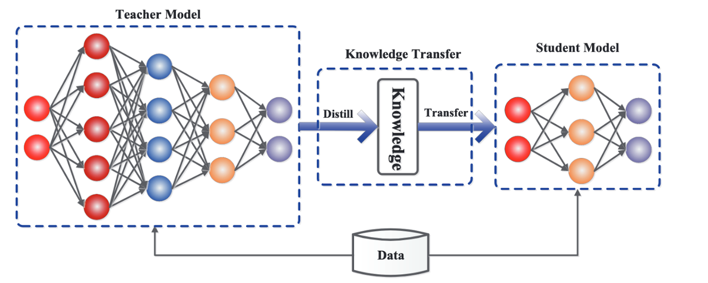
<p>Model distillation trains a smaller model (student model) to approximate a larger model (teacher model), effectively transferring knowledge from the larger model to the smaller one and reducing the smaller model’s parameters. For LLMs, this approach is particularly useful since they contain billions of parameters and are inherently “capable” of various tasks.</p>

<p><img src="https://s2.loli.net/2024/11/07/qTWs7P4mpLrOIHv.png" alt="" /></p>

<p>One distillation method uses LLMs for labeling unlabeled data on a specific task, which can then train a smaller task-specific model. This method is straightforward but requires substantial unlabeled data and training time. Notably, many GenAI companies (like OpenAI) explicitly prohibit using their models’ generated data to train competitors’ models.</p>

<p>Another popular distillation method is Knowledge Distillation (e.g., DistilBERT), where a smaller model (student) is trained to approximate the output probability distribution of a larger model (teacher). This approach focuses only on the teacher model’s output distribution, not the specific values. However, since it requires the LLM’s full output probability distribution, it can only be performed on open-source LLMs.</p>

<h3 id="decoding">Decoding</h3>

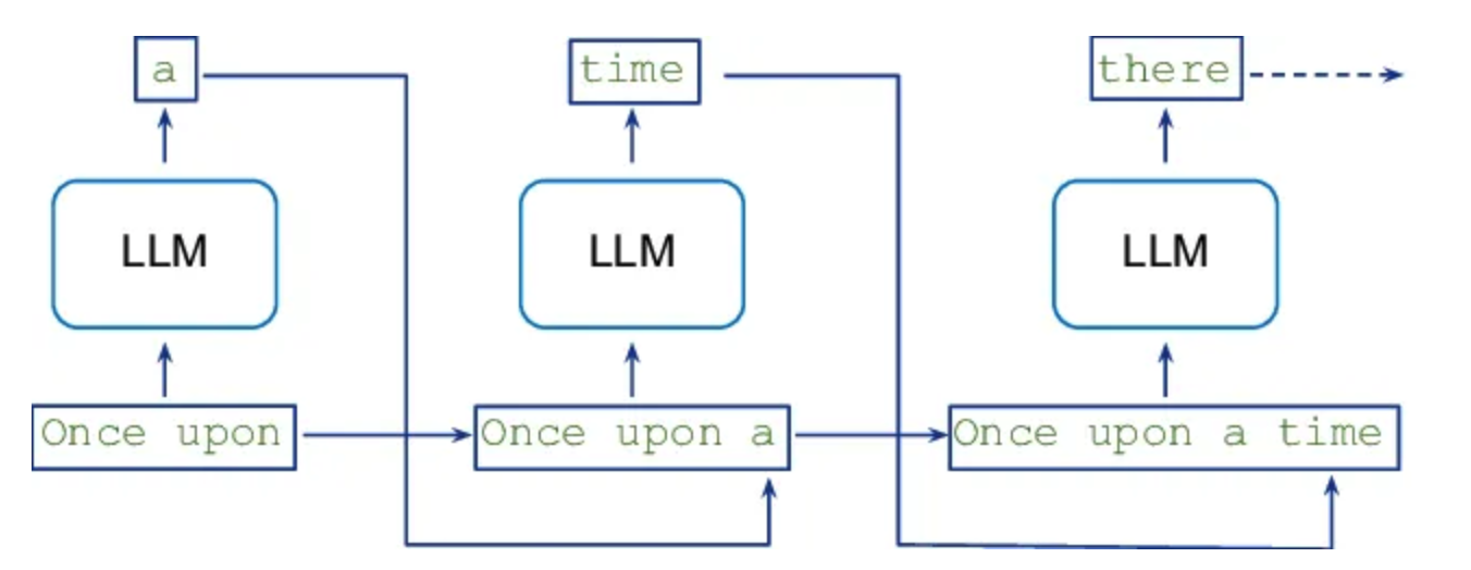
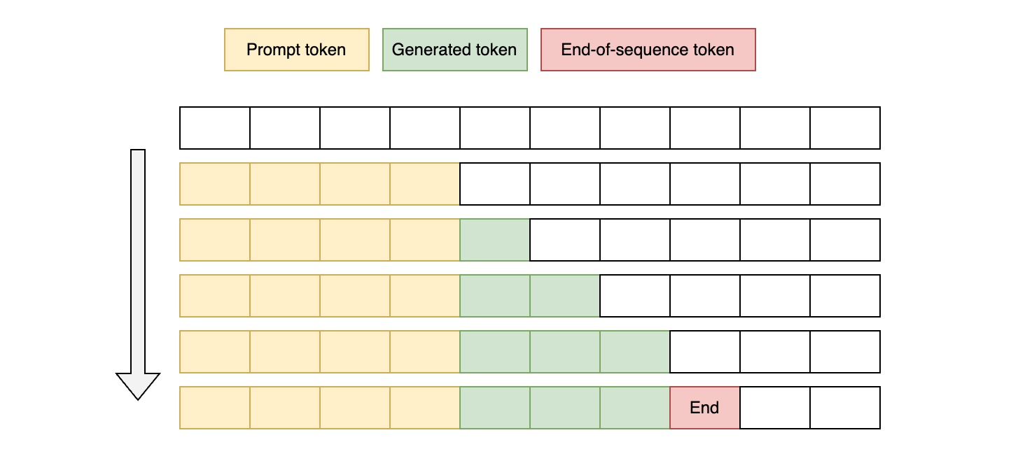
<p>Decoding speed directly affects LLM inference speed, so several decoding optimization methods exist for LLMs. Traditional LLMs perform inference using autoregressive sampling (as shown below).</p>

<p><img src="https://s2.loli.net/2024/11/07/x9vCILhiaquSjRG.png" alt="" /></p>

<p>This structure introduces time dependencies in model inference.</p>

<h4 id="non-autoregressive-nar-decoding">Non-autoregressive (NAR) Decoding</h4>

<p>The term “Autoregressive” refers to the use of previous time steps to predict the current output. Non-autoregressive decoding generates all outputs simultaneously without depending on prior outputs, effectively removing dependencies between tokens and allowing parallel generation. This method significantly reduces decoding time but may decrease model accuracy.</p>

<h4 id="speculative-decoding">Speculative Decoding</h4>

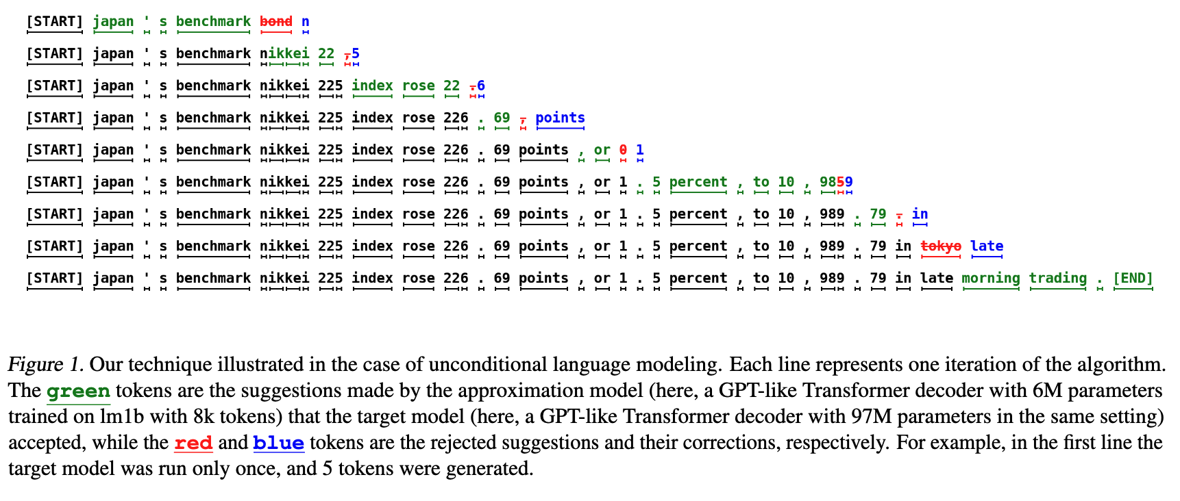
<p>Speculative Decoding, also known as assisted generation or Medusa, increases LLM inference throughput (~2-3x) with minimal accuracy loss. It requires one or more smaller models to assist LLM inference:</p>

<ul>
  <li>Target Model: The primary LLM we use</li>
  <li>Small Draft (Approximation) Model: A lighter model primarily for speeding up inference</li>
</ul>

<p><img src="https://s2.loli.net/2024/11/07/2QGv5nhecj4lFfs.png" alt="" /></p>

<p>During inference, the Small Draft Model generates a draft output, which the Target Model refines. This approach speeds up inference by generating multiple tokens in a single LLM forward pass. Here is the general workflow (<a href="https://arxiv.org/pdf/2302.01318">Google DeepMind</a>):</p>

<ul>
  <li>Step 1: Auto-regressive decode \(K\) tokens from <strong>draft model</strong> and get final \(p\), append \(K\) new tokens into input \(x\).</li>
  <li>Step 2: <strong>Target model</strong> forward passes on the \(x\) to get the probability distribution \(q\) of all tokens.</li>
  <li>Step 3: Compare the probability \(q\) and \(p\) to decide whether the token should be kept or rejected. Sample a new token (and its afterward tokens) once rejected.</li>
  <li>Step 4: If all tokens are accepted, sample the next token (based on the token distribution).</li>
  <li>Step 5: loop the process for \(K\) tokens as a pass. The larger \(K\) is the faster inference speedup, the lower latency gain.</li>
</ul>

<p>Usually, if the target model’s token probability is higher than the draft model’s under a certain tokend, we will accept the token. Like the table shown below:</p>

<table>
  <thead>
    <tr>
      <th>Token</th>
      <th>I</th>
      <th>like</th>
      <th>eat</th>
      <th>apple</th>
      <th>pie</th>
      <th>.</th>
    </tr>
  </thead>
  <tbody>
    <tr>
      <td>Draft Model p(x)</td>
      <td>0.8</td>
      <td>0.7</td>
      <td>0.9</td>
      <td>0.8</td>
      <td>0.7</td>
      <td>0.6</td>
    </tr>
    <tr>
      <td>Target Model q(x)</td>
      <td>0.9</td>
      <td>0.8</td>
      <td>0.8</td>
      <td>0.3</td>
      <td>0.8</td>
      <td>0.4</td>
    </tr>
    <tr>
      <td>Accept</td>
      <td>Yes</td>
      <td>Yes</td>
      <td>8/9</td>
      <td>3/8</td>
      <td>Yes</td>
      <td>4/6</td>
    </tr>
  </tbody>
</table>

<p>You can see we use the \(\frac{q(x)}{p(x)}\) to decide whether to accept the token or not. If a token is rejected, the rest of the tokens in a total \(K\) will be re-sampled. As you know, based on the above table, the acceptance rate is the key to improve the inference speedup of speculative decoding. If the draft yields tokens that are totally different from the target model, the acceptance rate will be low, and the inference speedup will be limited.</p>

<p>To analyze Speculative Decoding’s performance, suppose the worst case where the draft model’s output is entirely wrong, necessitating corrections by the target model each time. In this case, the inference count will not exceed that of autoregressive decoding. However, if the draft model generates satisfactory values, multiple draft tokens can be validated in a single target model pass, significantly increasing speed.</p>

<p>🔴 <strong>Choosing the Right Draft Model</strong></p>

<p>The draft model selection is crucial for speculative decoding. There are few key points to consider:</p>

<ul>
  <li>Target model is larger than the draft model too much: the rejection rate is high, results in the low efficiency.</li>
  <li>Both models are too small: the performance difference between is not large enough to accelerate the inference.</li>
  <li>The two models are pre-trained with different vocabularies: the candidate distribution is different from the target distribution, the rejection rate is high.</li>
</ul>

<p>For example, if you are serving <code class="language-plaintext highlighter-rouge">LLama3-70b</code>, it is better to use a <code class="language-plaintext highlighter-rouge">LLama3-7b</code> as the draft model, rather than another 70b model or other models trained with different vocabularies.</p>

<p>🔴 <strong>Spectulative Decoding w/o Draft Models</strong></p>

<p>Since it is so hard to select or train a draft model, many researches are trying to eliminate the draft model. Here are some methods:</p>

<ul>
  <li><a href="https://huggingface.co/docs/text-generation-inference/en/conceptual/speculation"><strong>N-gram</strong></a>: Without a new draft model, take a look back of the historical generated distribution vocabulary, pick the top-n for the next draft.</li>
  <li><a href="https://arxiv.org/abs/2401.10774"><strong>Medusa</strong></a>: Using extract decoding head for draft generation, without extra model.</li>
  <li><a href="https://arxiv.org/abs/2402.02057"><strong>Lookahead</strong></a>: Using Jacobi decoding to guess multiple n-grams in a pass (in parallel using GPU).</li>
  <li><a href="https://arxiv.org/abs/2401.15077"><strong>EAGLE</strong></a>: Similar to Medusa, but using a auto-regression head to predict the draft from feature-level instead of token-level. Which is more accurate, results in a higher acceptance rate.</li>
</ul>

<h3 id="batching">Batching</h3>

<p>Batching is a vital optimization method in model inference. By processing multiple input data instances simultaneously, batching maximizes parallel computation, enhancing GPU utilization and increasing inference throughput.</p>

<h4 id="static-batching">Static Batching</h4>

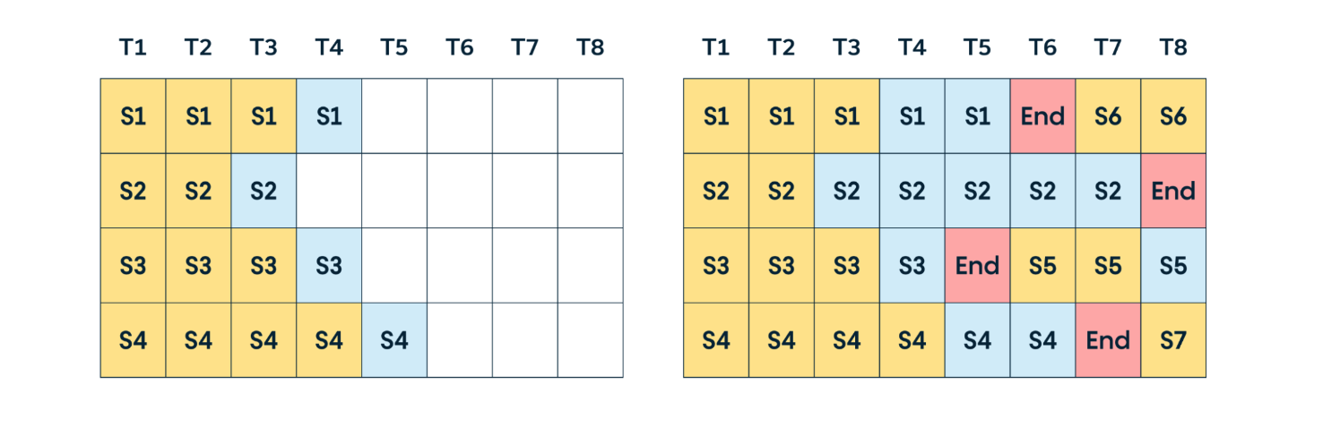
<p>Static batching refers to processing multiple input data instances simultaneously during inference. This approach reduces computation and speeds up inference but requires predefined input sizes. For inputs of different sizes, padding may be necessary.</p>

<p>A simple example is shown below:</p>

<p><img src="https://s2.loli.net/2024/11/08/BxFl9jOnZYQDcpC.png" alt="" /></p>

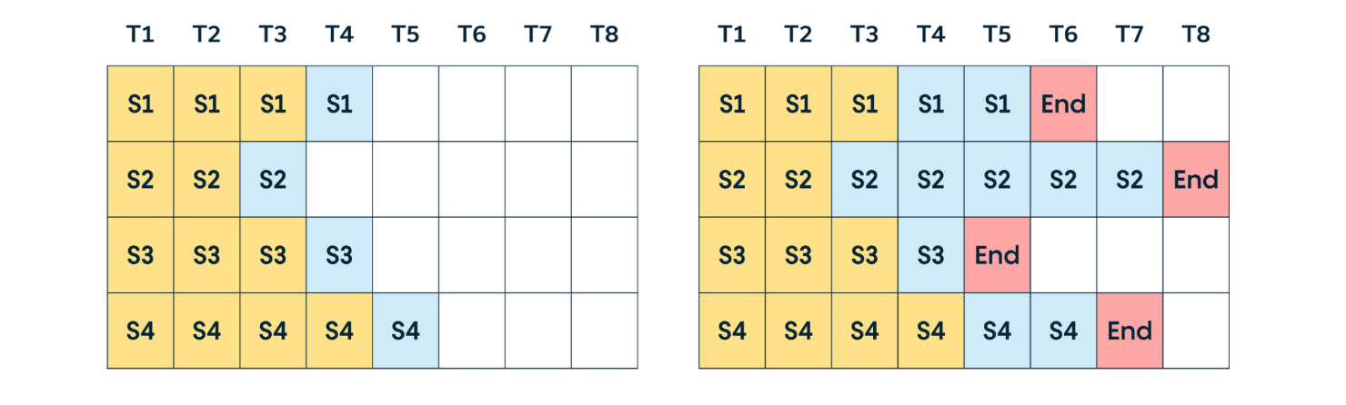
<p>Static batching waits for the “longest” request to finish before returning results. This can lead to extended waiting times for some requests, limiting GPU utilization. Moreover, with a small workload, static batching might cause queuing delays as it waits for enough requests to reach the batch size, further reducing GPU utilization.</p>

<h4 id="continuous-batching">Continuous Batching</h4>

<p>To address the waiting issue in static batching, continuous batching returns completed requests first, continuing inference for other requests. A visual example is below:</p>

<p><img src="https://s2.loli.net/2024/11/08/zsPJp3I9lTLGNyS.png" alt="" /></p>

<p>However, a potential issue with this approach is the need to pre-allocate “sufficient” memory space to handle the longest request in each batch to prevent memory overflow. This can lead to memory waste, as the size of incoming requests is unknown in advance. This is why PagedAttention is used to optimize LLM memory management, which we’ll discuss later.</p>

<h3 id="memory-optimization">Memory Optimization</h3>

<p>The attention mechanism is central to LLMs, enabling them to weigh input data parts differently and focus on relevant information for a task. Improving attention performance enhances inference speed while reducing computation. Since attention is memory-bound, memory management optimization is crucial.</p>

<p>LLM inference memory allocation breakdown:</p>

<ul>
  <li>Model Parameters: About 65%-70%</li>
  <li>KV Cache: Stores the key and value of the autoregressive model, about 25%-30%</li>
  <li>Others: Activations, intermediate results, about 5%-10%</li>
</ul>

<p>A simplified version of LLM memory usage during inference:</p>

<p><img src="https://s2.loli.net/2024/11/07/LIz348WBD2TZE5H.png" alt="" /></p>

<p>LLM inference consists of two phases:</p>

<ul>
  <li>Prefill phase: Prompt token preloading and input computation</li>
  <li>Decode phase: Generation of each subsequent token</li>
</ul>

<p>During the prefill phase, LLM precomputes inputs that remain constant in subsequent generations, leveraging GPU parallelism.</p>

<h4 id="flashattention-gpu-only">FlashAttention (GPU only)</h4>

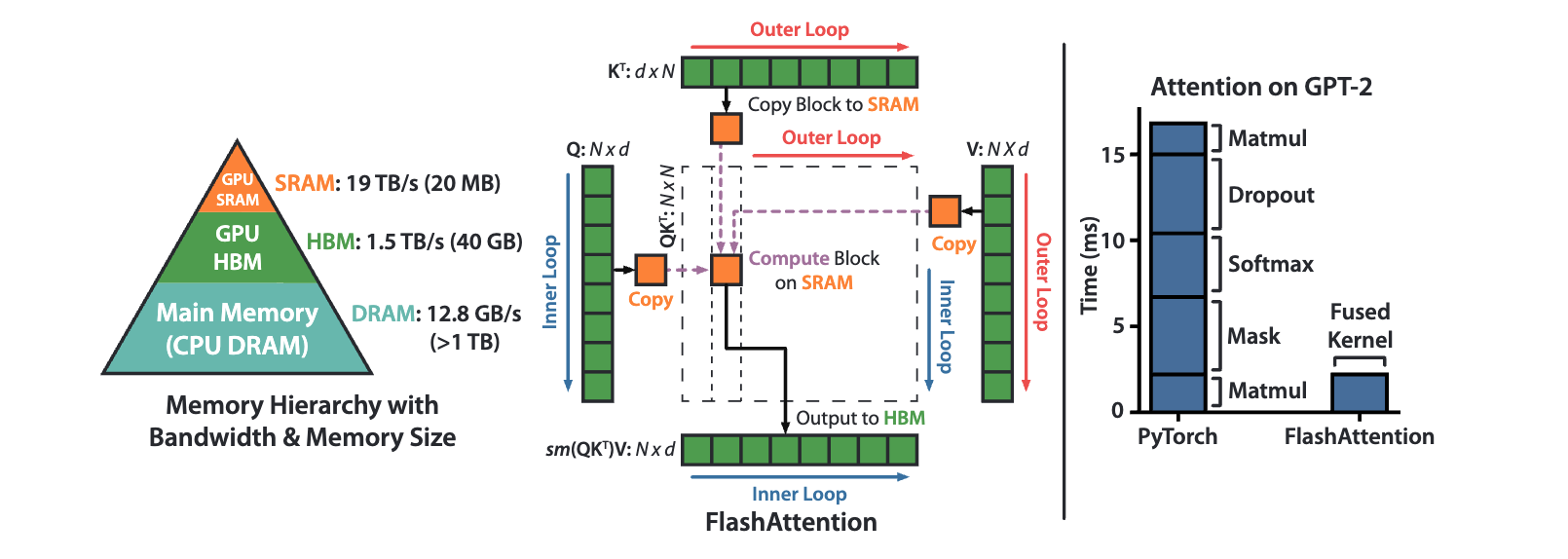
<p>Regardless of memory type, a general rule is that faster memory is more expensive and has less capacity. FlashAttention uses three types of memory (a sample configuration on an Nvidia A100 + CPU machine):</p>

<ul>
  <li>CPU main memory (CPU DRAM): Largest capacity, slowest speed (12.8GB/s, &gt;1TB)</li>
  <li>HBM (high bandwidth memory): Fastest speed, moderate capacity (1.5TB/s, 40GB)</li>
  <li>SRAM (on-chip memory): Fastest, smallest capacity (19TB/s, 20MB)</li>
</ul>

<p>“Graphics memory” typically refers to HBM.</p>

<p><img src="https://s2.loli.net/2024/11/07/FbE1QJRkDVPZTic.png" alt="" /></p>

<p>Traditional Transformer inference follows these steps, assuming \(K, V, Q \in R^{N \times d}\) matrices in HBM:</p>

<ul>
  <li>Load \(Q\) and \(K\) by blocks from HBM, compute \(S = QK^T\) and store \(S\) in HBM.</li>
  <li>Read \(S\) from HBM, compute \(P = \text{softmax}(S)\), and store \(P\) in HBM.</li>
  <li>Load \(P\) from HBM, compute \(O = PV\), and store \(O\) in HBM.</li>
  <li>Return \(O\)</li>
</ul>

<p>Here, \(K, V, Q\) are key, value, and query matrices, \(S\) is the score matrix, \(P\) is the softmax probability matrix, and \(O\) is the output matrix. The traditional Transformer loads all QKV matrices into HBM for matrix multiplication, which increases HBM read/write operations and reduces inference speed.</p>

<p>The intermediate storage of \(S\) between the first and second steps is unnecessary. If \(S\) is cached in SRAM, HBM read/write operations can be reduced. This approach, known as kernel fusion on GPUs, merges low-level computations to reduce communication overhead. However, SRAM’s limited capacity prevents it from storing the entire \(S\) matrix. FlashAttention addresses this issue with two key ideas:</p>

<ul>
  <li><strong>Tiling</strong>: Used in both forward and backward passes by chunking the NxN softmax/scores matrix into blocks, each small enough for SRAM.</li>
  <li><strong>Recomputation</strong>: Used only in the backward pass. This approach stores outputs and softmax normalization statistics to recompute attention matrices, using incremental calculation to obtain precise attention outputs.</li>
</ul>

<h4 id="pagedattention">PagedAttention</h4>

<p>According to our earlier analysis of LLM memory structures, the KV Cache occupies significant memory, making it a primary target for optimization.</p>

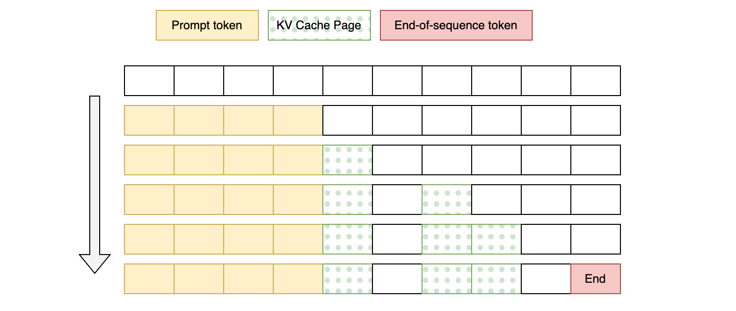
<p>PagedAttention, a <a href="https://docs.vllm.ai/en/v0.6.0/dev/kernel/paged_attention.html">vLLM</a> optimization inspired by the “virtual memory with paging” concept in traditional OS memory management, divides the KV cache into non-contiguous, fixed-size pages. During inference, only the necessary pages are loaded as needed.</p>

<p><img src="https://s2.loli.net/2024/11/07/qrol6uyYREKFnJ1.png" alt="" /></p>

<p>This approach eliminates the need to pre-allocate continuous memory space for the maximum context length and dynamically loads KV cache pages during inference to improve efficiency. However, this method does not guarantee perfect memory utilization; the last block after paging may be partially wasted (vLLM currently achieves less than 4% waste).</p>

<h3 id="parallelism">Parallelism</h3>

<p>Parallel computing is a crucial method for speeding up model inference by dividing the computation into multiple parts for simultaneous execution. Common parallel computing methods include data parallelism, model parallelism, tensor parallelism, and pipeline parallelism. While parallelism is widely used in both model training and inference, Tensor and Pipeline parallelism are more common in inference due to the smaller computation load, more complex data pipeline, and need to handle production uncertainties.</p>

<h4 id="tensor-parallelism">Tensor Parallelism</h4>

<p>Tensor parallelism uses multiple GPUs for distributed matrix computation. In LLM inference, tensor operations mainly refer to matrix multiplications of the Key, Value, and Query matrices in the attention mechanism and MLP layers. Matrix multiplications are split across GPUs to utilize multiple devices.</p>

<p>For example, with input vector \(X\), weight matrix \(A\), and output vector \(Y\), we can split the calculation across 3 GPUs as follows:</p>

\[Y = X \cdot A\]

<p>is equivalent to</p>

\[\begin{bmatrix} Y_1 \\ Y_2 \\ Y_3 \end{bmatrix} = X \cdot \begin{bmatrix} A_1 &amp; A_2 &amp; A_3 \end{bmatrix}\]

<p>where each \(Y_i = X \cdot A_i\) is computed on a separate GPU.</p>

<h4 id="pipeline-parallelism">Pipeline Parallelism</h4>

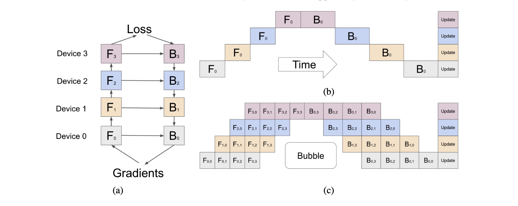
<p>Pipeline parallelism involves dividing the model vertically into chunks, each allocated to a different device (stage) for computation. During forwarding, each stage passes intermediate activations to the next stage for parallel computation.</p>

<p><img src="https://s2.loli.net/2024/11/08/UhZdXfrLaDGHQNM.png" alt="" /></p>

<p>Due to the need for sequential activation transfer and processing across pipeline stages, certain devices idle while awaiting the previous stage’s computation results, reducing pipeline parallelism efficiency, known as “pipeline bubbles.”</p>

<p>Microbatching can reduce pipeline bubbles by dividing input data into smaller batches and interleaving them across stages, reducing waiting times. However, this does not entirely eliminate pipeline bubbles.</p>

<h3 id="reference">Reference</h3>

<p>Some of the pictures/links are from the following articles:</p>

<ul>
  <li><a href="https://arxiv.org/abs/2211.17192">Fast Inference from Transformers via Speculative Decoding</a></li>
  <li><a href="https://towardsdatascience.com/model-compression-via-pruning-ac9b730a7c7b">Model Compression via Pruning</a></li>
  <li><a href="https://snorkel.ai/blog/llm-distillation-demystified-a-complete-guide/">LLM distillation demystified: a complete guide</a></li>
  <li><a href="https://www.datacamp.com/blog/distillation-llm">LLM Distillation Explained: Applications, Implementation &amp; More</a></li>
  <li><a href="https://arxiv.org/abs/2205.14135">FlashAttention: Fast and Memory-Efficient Exact Attention with IO-Awareness</a></li>
  <li><a href="https://github.com/vllm-project/vllm">vLLM: A high-throughput and memory-efficient inference and serving engine for LLMs</a></li>
  <li><a href="https://www.run.ai/blog/serving-large-language-models">What it means to serve an LLM and which serving technology to choose from</a></li>
  <li><a href="https://developer.nvidia.com/blog/mastering-llm-techniques-inference-optimization/">Mastering LLM Techniques: Inference Optimization</a></li>
  <li><a href="https://arxiv.org/abs/1811.06965">GPipe: Efficient Training of Giant Neural Networks using Pipeline Parallelism</a></li>
  <li><a href="https://arxiv.org/abs/2312.15234">Towards Efficient Generative Large Language Model Serving: A Survey from Algorithms to Systems</a></li>
  <li><a href="https://arxiv.org/abs/2204.02311">PaLM: Scaling Language Modeling with Pathways</a></li>
  <li><a href="https://arxiv.org/abs/2401.10774">Medusa: Simple LLM Inference Acceleration Framework with Multiple Decoding Heads</a></li>
  <li><a href="https://arxiv.org/abs/2402.02057">Break the Sequential Dependency of LLM Inference Using Lookahead Decoding</a></li>
  <li><a href="https://arxiv.org/abs/2401.15077">EAGLE: Speculative Sampling Requires Rethinking Feature Uncertainty</a></li>
  <li><a href="https://pytorch.org/blog/quantization-aware-training/">Quantization-Aware Training for Large Language Models with PyTorch</a></li>
</ul>]]></content><author><name>Yizheng</name></author><category term="tech" /><summary type="html"><![CDATA[Table of Contents]]></summary></entry><entry><title type="html">写在第二次骨折后</title><link href="https://blog.huangyz.name//life/2024/07/08/note.html" rel="alternate" type="text/html" title="写在第二次骨折后" /><published>2024-07-08T00:00:00+00:00</published><updated>2024-07-08T00:00:00+00:00</updated><id>https://blog.huangyz.name//life/2024/07/08/note</id><content type="html" xml:base="https://blog.huangyz.name//life/2024/07/08/note.html"><![CDATA[<p>三周前，因为在攀岩的过程中不慎掉落，我又把左胳膊肘摔断了，去医院检查说是肘关节脱臼加上桡骨小头骨折，韧带断裂。为什么说“又”呢，是因为我非常清楚地记得 12 年前，因为一个落地不稳的前空翻，我把右脚脚掌的五根趾骨都给拧断了，为此我度过了人生中最痛苦，也是最印象深刻的半年。还记得受伤的时候是九月份，我刚开始上高中，刚加入足球队，一切都是那么的充满希望。右脚的骨折却给了我当头一棒，当时坐着轮椅在医院的我拼命询问着医生能不能恢复到从前，医生说：“你的脚掌就像一个碗，我现在给它摔碎了再用胶水粘起来，能和以前一样吗？”。</p>

<p>我当时心里难受的像是被人判了死刑。</p>

<p>人是很脆弱的，短短几秒的一个失误，就让你用以年月的时间来治愈。还记得当时住校在 5 楼，拄着拐杖上楼成为了那时最大的梦魇。每次洗澡需要用保鲜膜将脚上的石膏一层层包裹着，生怕沾到水了以后在南方的潮湿天气下发霉。卫生间的厕所没有马桶，因为一条腿根本没办法蹲下去，于是便和室友从音乐教室偷了把椅子，上面拿链锯掏了个洞，自顾自地给卫生间 “改装” 了一下，没想到还意外的好用。另外，骨折往往伴随着肿胀，病人一般需要把脚 “架高” 来缓解由于血液下流导致肿胀加重，所以那时候的上课必须把脚架在桌子上，然后手从裤裆下写字，听起来感觉有些滑稽，不过个中辛苦也只有自己能够体会。总之，那是一段痛苦的日子，无数个因为疼痛而无法入眠的冬夜，生活好像变得一团糟，学习也变得一团糟。</p>

<p>不过放眼 12 年后一切又显得那么的微不足道，现在我时常忘记自己当初受伤的是哪只脚，而且每每回想起来，那段日子也并不是只有痛苦和焦虑，似乎也有不少有趣的时刻：比如受伤后的第一个生日收到了全班每人签名祝福的手绘海报；比如受伤两个月后我顺利成为了全校 “三条腿跑步最快的人”（两条拐+一只脚）；比如因为没有办法进行户外运动而开始拧魔方一样（后来居然还拿了大学魔方比赛的冠军）。生活中的很多乐趣并不是右脚掌带给你的，只是作为一个健康健全的人，往往会忽视自己原来有那么多的时间可以利用，却不知道浪费在了什么地方，人自己能够从那么多的点滴中汲取快乐，却还是要寻找焦虑与不愉快。所以骨折后那段漫长的愈合，我感觉不仅仅愈合了骨头之间的伤口，也在一定程度上愈合了人那浮躁不满的内心。</p>

<p>有人问：“你会不会后悔当时做出那个空翻/攀那条攀岩线路的决定？”，我觉得不后悔是假的，非常后悔，因为手脚的不便以及后续的康复是个痛苦而漫长的过程。但是你问我下次还会不会去做这么个运动？我会，并且康复中的焦虑很大程度上是源于对自己没办法继续享受某项活动的恐惧。余华说：“活着就是为了活着本身，而不是活着之外的的任何事物”，没有人为了不受伤而跑酷攀岩，毕竟 life is taking risks，即使运气不好受伤了，那也是属于自己的一种体验。于是在这次受伤之后，我放平了心态，带着十多年前修炼的那套苦中作乐的传统艺能，决定体会当下，静心复盘。好在这次受伤不像之前那么严重，在熬过了第一周淤血肿胀之后，医生给我配了一副看着很赛博的机械护具（看着还蛮酷的，朋友说因祸得福弄了件时尚单品）。恰好室友和同学大多都因为暑假离开了洛杉矶，整个世界仿佛因为手臂的折断安静了下来，属于我的空间由一个房间瞬间拓宽到了整栋楼。</p>

<p>这种感觉很像当初疫情最严重的时候，人与人之间的社交停留在了互联网，而绝大多数的时间都在和自己相处。由于没有了社交和户外活动，我开始把更多的时间放在做一些自己感觉舒服的事情上，比如做饭。Costco 买的菜分量真的很大，所以如果不做完就很容易坏，但是我感觉没有人会喜欢一直吃一种菜的做法，所以逼得你不得不整点花样：比如把喝不完的牛奶做成双皮奶，珍珠奶茶和烤牛奶布丁（另外安利 Ralphs 的甜茶，简直是做奶茶的神），把吃不完的吐司面包做成（不太正宗的）肉夹馍和牛肉汉堡，甚至用 “残存” 的一只好手练一下颠锅。很奇妙的一件事情是：在人并未受伤的时候，做什么事情都很快，但是很难去概括每一天都做了些什么，感觉浪费时间的部分比较多。但是当自己光是穿个袜子都要花五分钟的时候，世界慢下来了，但是它并没有停下来。该做的事情还是做了，甚至做得更多，感受更加充盈。这也让我开始反思过去一年的创业历程 – 或许冲的过快并不是一件好事。在去了湾区参观和交流以后，我发现硅谷的创业公司有一种很神奇的状态，一些工作状态非常松弛的公司往往还能做出非常惊艳和领先的产品，这和国内必须快人一等，使劲卷过其他人的思路很不一样，甚至有违常理：为什么不怎么努力，看着那么懒，却能成功？我觉得在第二次骨折的这段时间里，我慢慢理解了一点。</p>

<p>有人说：“世间所有的焦虑都来自于内心的不平衡”，在硅谷这个充满着机会，钱，和新的认知的地方，有能力的人很难不变的急躁：迫切地想要拿出成果，迫切地想要更多的证明自己，想要变得更快，不错过每个机会。但是骨折让一切慢了下来，在肉体努力康复的同时，它也给了一段和自我沟通的完美时间。身体能力的减弱逼迫着你减去生活中很多原本不需要的人际或者是事物，留下最重要的东西。特别在这个物欲横流的年代，难的不是既要又要，而是做减法，偶尔停下来关注自己内心真正的感受，真正地爱自己。</p>

<p>慢慢来，反而有的时候更快一点。</p>

<p>很久没有在博客更新，也因为受伤的缘故能够有时间胡乱地记录一下内心所想。希望能够早日康复，与君共勉。</p>]]></content><author><name>Yizheng</name></author><category term="life" /><summary type="html"><![CDATA[三周前，因为在攀岩的过程中不慎掉落，我又把左胳膊肘摔断了，去医院检查说是肘关节脱臼加上桡骨小头骨折，韧带断裂。为什么说“又”呢，是因为我非常清楚地记得 12 年前，因为一个落地不稳的前空翻，我把右脚脚掌的五根趾骨都给拧断了，为此我度过了人生中最痛苦，也是最印象深刻的半年。还记得受伤的时候是九月份，我刚开始上高中，刚加入足球队，一切都是那么的充满希望。右脚的骨折却给了我当头一棒，当时坐着轮椅在医院的我拼命询问着医生能不能恢复到从前，医生说：“你的脚掌就像一个碗，我现在给它摔碎了再用胶水粘起来，能和以前一样吗？”。]]></summary></entry><entry><title type="html">Lifelong Learning in Modern AI Systems</title><link href="https://blog.huangyz.name//tech/2023/12/09/notes.html" rel="alternate" type="text/html" title="Lifelong Learning in Modern AI Systems" /><published>2023-12-09T00:00:00+00:00</published><updated>2023-12-09T00:00:00+00:00</updated><id>https://blog.huangyz.name//tech/2023/12/09/notes</id><content type="html" xml:base="https://blog.huangyz.name//tech/2023/12/09/notes.html"><![CDATA[<h3 id="table-of-contents">Table of Contents</h3>

<ul>
  <li><a href="#what-is-lifelong-learning">What is Lifelong Learning?</a></li>
  <li><a href="#methods-of-lifelong-learning">Methods of Lifelong Learning</a>
    <ul>
      <li><a href="#regularization-based-methods">Regularization-based Methods</a></li>
      <li><a href="#replay-based-methods">Replay-based Methods</a></li>
      <li><a href="#dynamic-expansion-methods">Dynamic Expansion Methods</a></li>
    </ul>
  </li>
  <li><a href="#continuous-learning-in-ai-systems">Continuous Learning in AI Systems</a>
    <ul>
      <li><a href="#better-monitoring">Better Monitoring</a></li>
      <li><a href="#better-model-deployment">Better Model Deployment</a></li>
      <li><a href="#learning-on-edge-devices">Learning on Edge Devices?</a></li>
      <li><a href="#large-scale">Large-scale?</a></li>
    </ul>
  </li>
</ul>

<h3 id="what-is-lifelong-learning">What is Lifelong Learning?</h3>

<p>Lifelong/Continual learning is often defined as an academic term. In the field of machine learning, it typically refers to continuously training a pre-trained model \(M_{ori}\) on new tasks \({t_1, t_2, ..., t_n}\) while maintaining high accuracy. This learning approach differs from traditional machine learning tasks, which are usually trained on a fixed dataset and tested on another fixed dataset. In such cases, the model’s performance often declines over time or due to changes in the test dataset (data drift).</p>

<p>According to this definition, lifelong learning has two main AI metrics:</p>

<ul>
  <li><strong>Task Performance</strong>: The performance of the model on new tasks, often measured by \(ACC\) (global accuracy) and \(ACC_t\) (accuracy of task \(t\)).</li>
  <li><strong>Catastrophic Forgetting</strong>: Whether the model forgets previously learned tasks when learning new ones. This is often measured using \(BWT\) and \(BWT_t\) (the loss in \(ACC\) after learning task \(t\)).</li>
</ul>

<p>From a systems perspective, additional metrics to consider include:</p>

<ul>
  <li><strong>Training-Time</strong>: The per-epoch average training time for all tasks.</li>
  <li><strong>Extra Parameters</strong>: The additional parameters introduced by the lifelong/continual learning strategy.</li>
  <li><strong>Buffer Size</strong>: The additional in-memory cache used by the strategy for storing replay data or model weights.</li>
</ul>

<p>Depending on the type of task, traditional lifelong learning can be further divided into:</p>

<ul>
  <li><strong>Class-change</strong>: A new task adds new classes to the overall task.</li>
  <li><strong>Distribution-change</strong>: A new task changes the data of one or more classes, affecting data distribution.</li>
  <li><strong>Task-change</strong>: The definition of the task changes with each new learning task.</li>
</ul>

<p>This is a straightforward and accurate problem definition, but in actual production environments, lifelong learning usually comes with more constraints and requires more engineering implementation details.</p>

<h3 id="methods-of-lifelong-learning">Methods of Lifelong Learning</h3>

<p>In the past few years, the AI research community has proposed many methods to address the problem of lifelong learning (mainly catastrophic forgetting). These methods can be categorized into three types:</p>

<h4 id="regularization-based-methods">Regularization-based Methods</h4>

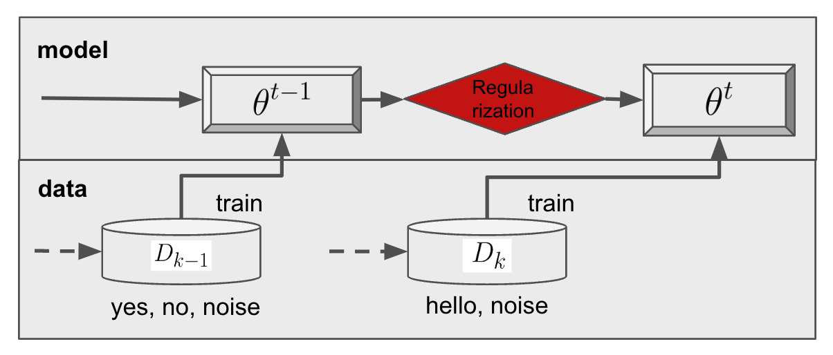
<p>Regularization-based methods involve adding constraints to the loss function to protect pre-trained parameters from being affected by new training tasks. Examples include Elastic Weight Consolidation (EWC), Synaptic Intelligence (SI), and Path Integral (PI).</p>

<p><img src="https://s2.loli.net/2024/11/05/AUri61PjqVIcSHl.png" alt="regularization-based" /></p>

<p>Specifically, the loss function for such methods is typically formulated as:</p>

\[\mathcal{L}' = \mathcal{L}(F_t(x_t;\theta^t), y_t) + \frac{\lambda}{2} \sum_{i} \Omega^t_i (\theta_i^t - \theta_i^{(t-1)})^2\]

<p>where \(\mathcal{L}\) is the loss function for task \(t\), \(\theta^t\) represents the parameters for task \(t\), \(\Omega^t_i\) represents the importance of parameter \(\theta_i^t\), and \(\lambda\) is a hyperparameter. The advantage of this method is that it does not require extra memory for storing data and is computationally efficient. However, it requires information from the previous task’s parameters and tuning the hyperparameter \(\lambda\). The effectiveness of this approach diminishes as the number of tasks increases due to the limited model parameters being unable to accommodate an infinite number of tasks.</p>

<h4 id="replay-based-methods">Replay-based Methods</h4>

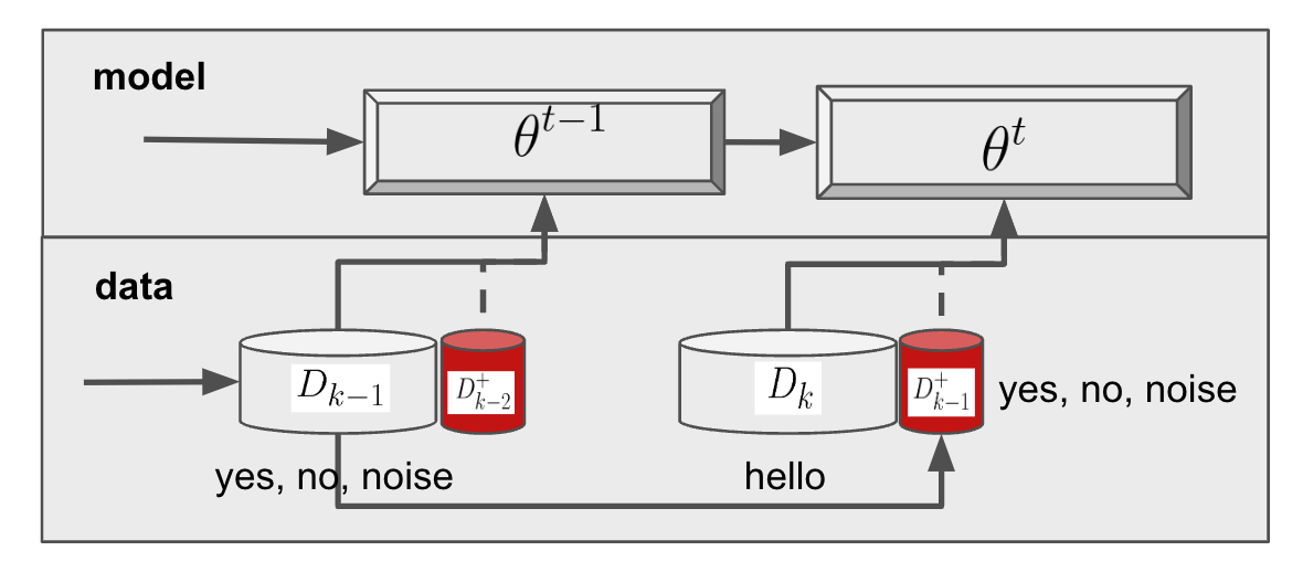
<p>This method avoids catastrophic forgetting by saving historical data or models. Examples include Naive Rehearsal (NR), Gradient Episodic Memory (GEM), and Meta-Experience Replay (MER).</p>

<p><img src="https://s2.loli.net/2024/11/05/Ib8E3HPh2DB145s.png" alt="replay-based" /></p>

<p>The advantage of this method is that it does not require additional constraints on model parameters. However, it increases memory usage and computational resources as historical data grows with the number of tasks. Selecting high-quality data for the model to “review” is also an important challenge.</p>

<h4 id="dynamic-expansion-methods">Dynamic Expansion Methods</h4>

<p>Dynamic expansion methods differ from the previous ones by dynamically increasing the model’s capacity to adapt to new tasks. Examples include Progressive Neural Networks (PNN) and Dynamic Expandable Network (DEN). By dynamically increasing model capacity, the model can better adapt to new tasks while keeping the parameters for old and new tasks separate to reduce catastrophic forgetting.</p>

<p>The advantage of this method is that it handles new tasks effectively but adds more parameters and computational complexity. Lifelong learning is limited by the finite capacity of the model.</p>

<h3 id="continuous-learning-in-ai-systems">Continuous Learning in AI Systems</h3>

<p>Frequent paper reading reveals that besides lifelong/continual learning, there is also the concept of continuous learning. What’s the difference between them? Continuous learning is a broader term that not only refers to continually training a model on new tasks but also encompasses many system-level considerations, such as designing a continuous learning system for specific business needs, data pipeline design, model deployment and update strategies, and model monitoring and evaluation strategies.</p>

<p>In such problems, system design becomes crucial. For example, a recommendation system is a typical case of continuous learning. In recommendation systems, user behavior must be continuously learned, and the model updated regularly. The model continuously updates its weights through inference, making its design different from other lifelong learning tasks.</p>

<p>Reinforcement learning is also an example of lifelong learning. In reinforcement learning, the model interacts with the environment and learns new tasks continuously. However, the focus is on designing better strategies, reward functions, and exploration strategies, not on avoiding catastrophic forgetting of past tasks.</p>

<p>Another example is video stream analysis systems (e.g., <a href="https://arxiv.org/abs/2012.10557">Ekya NSDI’22, by Romil Bhardwaj et al.</a>). These systems inherently deal with time-series data without a fixed task dataset, requiring continual system updates to maintain high accuracy. Such models often run on edge devices, necessitating efficient cloud-edge collaboration and careful data caching due to limited data storage.</p>

<p>Limited by current model capabilities and evolving business requirements, today’s lifelong learning definitions and solutions still have a long way to go before achieving “AI self-evolution.” However, better system design can maximize the benefits of lifelong learning. The general process includes:</p>

<h4 id="better-monitoring">Better Monitoring</h4>

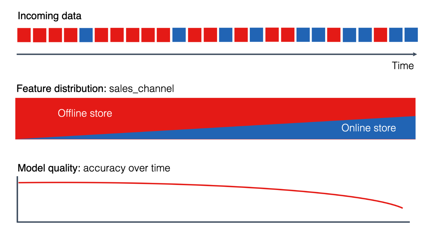
<p>To handle a continuously changing deployment environment, the system must first collect and analyze data to detect changes in both data and models. A drop in model performance due to data distribution changes should trigger model fine-tuning or retraining.</p>

<p><img src="https://s2.loli.net/2024/11/05/jh9NQUxlTFomW5f.png" alt="https://www.evidentlyai.com/ml-in-production/data-drift" /></p>

<p>Main drift detection methods include:</p>

<ul>
  <li><strong>Data Distribution Comparison</strong>: Regularly comparing new and old data distributions to detect changes.</li>
  <li><strong>Model Performance Monitoring</strong>: Regularly checking model performance and triggering fine-tuning or retraining if performance drops.</li>
</ul>

<h4 id="better-model-deployment">Better Model Deployment</h4>

<p>To adapt to a changing deployment environment, the system must be able to quickly deploy new models and roll back to previous versions when needed. This requires a hot-swapping system that does not disrupt online services. Conduct A/B testing beforehand to ensure the new model’s performance and safety.</p>

<p>In large-scale distributed systems, you can deploy a new model on a subset of nodes and gradually expand, minimizing risks if the deployment fails. Node selection, model gray release, and rollback strategies depend on specific business needs.</p>

<h4 id="learning-on-edge-devices">Learning on Edge Devices?</h4>

<p>Learning on edge devices is a good approach for preserving user data privacy while providing “personalized” services. However, it is limited by:</p>

<ul>
  <li><strong>Storage space</strong>: Edge devices have limited storage, so they cannot store large amounts of historical data or model parameters.</li>
  <li><strong>Computational resources</strong>: Edge devices have limited computing power, making large-scale model training infeasible and requiring fast model updates.</li>
</ul>

<p>A common solution is to design an efficient cloud-edge collaboration system. The cloud handles the base pre-trained model updates (usually monthly), while the edge device performs frequent model updates (daily). The edge device also needs an efficient data caching system to ensure sufficient training data without consuming excessive storage.</p>

<h4 id="large-scale">Large-scale?</h4>

<p>As model size (parameter count) increases, the cost of continuous learning rises, making it more challenging. Generally, larger models are better at generalizing to similar tasks, but they require more computation, data, and time to learn new tasks.</p>

<p>For large language models (LLMs), training involves more than simple data input and parameter updates—it is a comprehensive pipeline, including data preprocessing, pretraining, and post-training with Reinforcement Learning from Human Feedback (RLHF) and Alignment with Human Values (AHV). This makes retraining large models costly, and even fine-tuning requires significant resources. While leveraging LLMs’ in-context learning, prompt engineering, or using RAG can make models “adapt” to new tasks, updating the model’s structure and reducing system learning costs remain unsolved challenges.</p>

<p>One direct approach is to use the understanding and code-generation capabilities of LLMs to explore completing traditional ML tasks end-to-end. If feasible, small models generated from this approach could perform RAG or fine-tuning to reduce the cost of continuous learning. The next step would involve generative model updates using LLM-generated code to achieve true continuous learning.</p>]]></content><author><name>Yizheng Huang</name></author><category term="tech" /><summary type="html"><![CDATA[Table of Contents]]></summary></entry><entry><title type="html">Using Checkpoint Recovery in Large-Scale ML Training</title><link href="https://blog.huangyz.name//tech/2023/04/05/notes-ckpt.html" rel="alternate" type="text/html" title="Using Checkpoint Recovery in Large-Scale ML Training" /><published>2023-04-05T00:00:00+00:00</published><updated>2023-04-05T00:00:00+00:00</updated><id>https://blog.huangyz.name//tech/2023/04/05/notes-ckpt</id><content type="html" xml:base="https://blog.huangyz.name//tech/2023/04/05/notes-ckpt.html"><![CDATA[<h3 id="table-of-contents">Table of Contents</h3>

<ul>
  <li><a href="#introduction">Introduction</a></li>
  <li><a href="#checkpoint-recovery">Checkpoint Recovery</a></li>
  <li><a href="#checkpoint-mechanism-and-frequency">Checkpoint Mechanism and Frequency</a></li>
  <li><a href="#consistency-issues-with-checkpoints">Consistency Issues with Checkpoints</a></li>
  <li><a href="#reducing-checkpoint-system-overhead">Reducing Checkpoint System Overhead</a></li>
  <li><a href="#reference">Reference</a></li>
</ul>

<h3 id="introduction">Introduction</h3>

<p>When training LLMs or larger deep learning models, distributed GPU clusters and massive amounts of training and testing data are often used. The duration of the training process is also usually quite long. In such cases, if issues like network interruptions or machine failures occur during training, they can cause training interruptions, resulting in significant time and financial losses.</p>

<p>Common causes of training interruptions include:</p>

<ul>
  <li>Hardware failures (such as GPU crashes or breakpoints)</li>
  <li>System-level issues (like memory overflow, virtual service preemption, etc.)</li>
  <li>Software-level issues (like code bugs, data corruption, etc.)</li>
</ul>

<p>Therefore, in a large-scale machine learning training task, to increase the system’s fault tolerance, we need to introduce mechanisms to ensure the reliability of the training process. One important mechanism among these is <strong>checkpoint recovery</strong>.</p>

<h3 id="checkpoint-recovery">Checkpoint Recovery</h3>

<p>A checkpoint refers to periodically saving the model’s parameters, the state of the optimizer, and other status information during the training process. This way, if training is interrupted, the process can be resumed by loading the checkpoint, rather than starting from scratch.</p>

<p>Common checkpoint APIs include TensorFlow’s <code class="language-plaintext highlighter-rouge">tf.train.Checkpoint</code> and PyTorch’s <code class="language-plaintext highlighter-rouge">torch.save</code>. To implement checkpoint recovery, we not only need a high-level API but also a low-level storage system to store the checkpoint. This storage system needs to have the following features:</p>

<ul>
  <li><strong>High performance</strong>: The storage system should ensure efficient writing and reading of checkpoints.</li>
  <li><strong>High reliability</strong>: The storage system should ensure the checkpoint’s reliability, meaning that once written, the checkpoint will not be lost. Additionally, if the storage system fails, mechanisms like backups should be in place to recover the checkpoint.</li>
</ul>

<h3 id="checkpoint-mechanism-and-frequency">Checkpoint Mechanism and Frequency</h3>

<p>When designing and implementing a checkpoint recovery system, the most important considerations are the <strong>checkpoint mechanism and frequency</strong> —these depend on the nature of the training task, such as the task’s duration, the size of the training data, and the complexity of the task.</p>

<p>Common checkpointing mechanisms include:</p>

<ul>
  <li>Periodically saving checkpoints based on the number of training steps</li>
  <li>Periodically saving checkpoints based on training time</li>
  <li>Periodically saving checkpoints based on the number of epochs</li>
</ul>

<p><img src="https://s2.loli.net/2024/11/02/j5nzSJ7TBri8wCp.png" alt="recover time" /></p>

<p>If the training task involves a large amount of data but relatively few model computations (memory-bound models), we can periodically save checkpoints based on the number of training steps. This ensures a relatively high checkpoint frequency during training. Conversely, if the training task involves substantial model computations but relatively little data (compute-bound models), we can save checkpoints based on training time to ensure sufficient checkpoints are available for recovery.</p>

<h3 id="consistency-issues-with-checkpoints">Consistency Issues with Checkpoints</h3>

<p>Checkpointing introduces some consistency challenges, such as:</p>

<ul>
  <li>Consistency issues between checkpoints across different workers in a distributed training system</li>
  <li>Consistency between checkpoints and the training process</li>
</ul>

<p>In distributed systems, the checkpoint recovery approach will vary depending on the training method. Generally, each compute node needs to save checkpoints (whether in data parallelism or model parallelism). However, during recovery, we must consider how to maintain checkpoint consistency across nodes. How can we resume normal training when the number of workers changes? How can we quickly verify the validity of checkpoints? How can we synchronize checkpoints across workers?</p>

<p>The checkpoint recovery process must ensure the atomicity of checkpoints. Assuming the training process is uninterrupted and checkpoint saving is asynchronous, the training process may continue while the checkpoint is being saved, leading to inconsistencies between the checkpoint and the model in the training process. To address this issue, we can adopt the following strategies:</p>

<ul>
  <li>Use synchronous checkpoint saving, where training is paused (<strong>stall training</strong>) while the checkpoint is saved, and resume training only after the checkpoint save is complete.</li>
  <li>Use asynchronous checkpoint saving (<strong>snapshot and persist</strong>), where the training process continues while a snapshot of the model is taken and the model is localized (persist) asynchronously. During recovery, verification is required to ensure checkpoint consistency.</li>
</ul>

<h3 id="reducing-checkpoint-system-overhead">Reducing Checkpoint System Overhead</h3>

<p>The checkpoint mechanism introduces some additional overhead, such as I/O overhead and CPU overhead. For example, if a synchronous checkpoint save is used (stall training), the training process is paused while saving the checkpoint, reducing training efficiency. If asynchronous checkpoint saving is used, additional I/O overhead is introduced, which can also decrease training efficiency.</p>

<p>In summary, while checkpoint recovery increases system stability, it also reduces system efficiency—this is a clear trade-off. To reduce the checkpoint system overhead, we can adopt the following strategies:</p>

<ul>
  <li>Predict potential system failures and save checkpoints dynamically: for example, increase checkpoint frequency when the network is unstable or monitor the hard drive’s status, using a DNN-based predictive model to anticipate drive failures.</li>
  <li>Use a high-performance storage system: for example, use SSDs instead of HDDs to save checkpoints, or use a KV storage system rather than a file system to save checkpoints, and so on.</li>
</ul>

<h3 id="reference">Reference</h3>

<ul>
  <li>CheckFreq: Frequent, Fine-Grained DNN Checkpointing (FAST ‘21)</li>
  <li>Check-N-Run: a Checkpointing System for Training Deep Learning Recommendation Models (NSDI ‘22)</li>
</ul>]]></content><author><name>Yizheng Huang</name></author><category term="tech" /><summary type="html"><![CDATA[Table of Contents]]></summary></entry><entry><title type="html">Model Serving Performance Test - A Deep Dive</title><link href="https://blog.huangyz.name//tech/2021/05/26/notes.html" rel="alternate" type="text/html" title="Model Serving Performance Test - A Deep Dive" /><published>2021-05-26T00:00:00+00:00</published><updated>2021-05-26T00:00:00+00:00</updated><id>https://blog.huangyz.name//tech/2021/05/26/notes</id><content type="html" xml:base="https://blog.huangyz.name//tech/2021/05/26/notes.html"><![CDATA[<h3 id="table-of-contents">Table of Contents</h3>

<ul>
  <li><a href="#the-typical-model-serving-workflow">The Typical Model Serving Workflow</a></li>
  <li><a href="#metrics-for-model-serving">Metrics for Model Serving</a>
    <ul>
      <li><a href="#static-metrics">Static Metrics</a></li>
      <li><a href="#dynamic-metrics">Dynamic Metrics</a></li>
    </ul>
  </li>
  <li><a href="#obtaining-dynamic-metrics">Obtaining Dynamic Metrics</a></li>
  <li><a href="#simulating-real-world-workloads">Simulating Real-world Workloads</a>
    <ul>
      <li><a href="#block-requests-sending">Block Requests Sending</a></li>
      <li><a href="#multiple-concurrencies-requests-sending">Multiple Concurrencies Requests Sending</a></li>
      <li><a href="#poisson-distribution-generation">Poisson Distribution Generation</a></li>
      <li><a href="#utilization-awared-workload-generation">Utilization-awared Workload Generation</a></li>
      <li><a href="#deep-learning-tasks">Deep Learning Tasks</a></li>
    </ul>
  </li>
  <li><a href="#performance-analysis">Performance Analysis</a>
    <ul>
      <li><a href="#latency-and-throughput-visualization">Latency and Throughput Visualization</a></li>
      <li><a href="#kde-and-cdf-for-latency-distribution">KDE and CDF for Latency Distribution</a></li>
      <li><a href="#heatmap-for-different-machine-learning-models">Heatmap for Different Machine Learning Models</a></li>
      <li><a href="#roofline-model-analysis">Roofline Model Analysis</a></li>
      <li><a href="#pipeline-analysis">Pipeline Analysis</a></li>
      <li><a href="#analysis-on-optimizations">Analysis on Optimizations</a></li>
    </ul>
  </li>
  <li><a href="#trends-and-what-next">Trends and What Next</a></li>
  <li><a href="#references">References</a></li>
</ul>

<p>In real-world production environments, people care greatly about the online service performance of models (e.g., latency, throughput) and the degree of hardware utilization (e.g., compute utilization rate, memory usage), as well as the friendliness to business logic developers (e.g., system API design).</p>

<p>Therefore, optimizing inference before model deployment has recently become a hot research area. This mainly includes pruning, quantization, and various compilation optimizations, which are optimizations applied to the model itself. However, the performance of the entire serving system is not solely determined by the model itself. The performance of the entire system is affected by the model, the deployment framework, the hardware, and the business logic. Therefore, it is necessary to conduct comprehensive performance testing on the entire system to obtain a more scientific understanding of the system’s performance.</p>

<h3 id="the-typical-model-serving-workflow">The Typical Model Serving Workflow</h3>

<p>Let’s take a look at the typical model serving workflow with a client-server architecture:</p>

<p><img src="https://s2.loli.net/2024/12/14/CSxYNUAI8eTOiJr.png" alt="" /></p>

<p>The model checkpoints/weights are usually stored in a model repository, and the model serving framework loads the model from the repository to the target hardware. For example, from the local disk to the CPU memory or from the CPU memory into the GPU memory. After the serving framework is initialized, and the model is loaded into the framework. The serving framework is responsible for managing the model’s life cycle, including managing the inference workers/jobs and the hardware resources, and providing an API for the client to send requests.</p>

<p>When the serving servers are ready, we can use the client to send requests for inference. In the client-side, it may include a client-side request processing and batching. Usually, putting data processing in the client-side will require more processing time since the client-side is usually a mobile device or a web browser with limited computing resources. But in term of protecting user privacy, it is a good practice to do so.</p>

<p>When the server receives the request, it puts the request into a queue and waits for the inference worker to process it. The inference worker will load the model from the memory and execute the model inference. After the inference is done, the worker will send the result back to the client. Some serving systems (e.g., Nvidia Triton Inference Server, Tensorflow-serving) support dynamic batching, which introduces the batching process in the server-side.</p>

<h3 id="metrics-for-model-serving">Metrics for Model Serving</h3>

<p>Now, we understand the typical model serving workflow. Let’s talk about the metrics for model serving, the metrics to measure the performance can be categorized into two categories: static metrics and dynamic metrics.</p>

<h4 id="static-metrics">Static Metrics</h4>

<p>Static metrics are metrics that can be calculated theoretically or from the model and hardware specifications. These metrics include:</p>

<ul>
  <li>Model Tasks: Classification, Detection, Segmentation, etc.</li>
  <li>Model complexity: FLOPs (time), memory footprint (space)</li>
  <li>Hardware capability: FLOPS (theoretical compute capability), memory, bandwidth</li>
</ul>

<h4 id="dynamic-metrics">Dynamic Metrics</h4>

<p>Dynamic metrics are metrics that can only be obtained through real-world performance profiling. These metrics include:</p>

<p><strong>For model deployment framework (software):</strong></p>

<ul>
  <li>Latency (P50, P95, P99) (ms)</li>
  <li>Throughput (varying batch sizes) (req/sec)</li>
</ul>

<p><strong>For model acceleration hardware:</strong></p>

<ul>
  <li>Average hardware utilization (%)</li>
  <li>Average memory utilization (%)</li>
  <li>Energy consumption per inference (J)</li>
  <li>Carbon emissions per inference (mg)</li>
  <li>Cold start time (sec)</li>
  <li>System startup time (sec)</li>
</ul>

<p><strong>For the model service pipeline:</strong></p>

<ul>
  <li>Pre-processing latency (ms)</li>
  <li>Post-processing latency (ms)</li>
  <li>Transmission time (ms)</li>
</ul>

<p>Above metrics are mainly for serving AI models on the cloud. Similarly, for mobile devices (edge devices), inference systems pay more attention to model storage occupancy and battery consumption, so energy consumption and hardware utilization during inference should be the focus. Different systems require different analyses.</p>

<p>There are many excellent works for measuring the Deep learning model serving performance, including <a href="https://github.com/triton-inference-server/model_analyzer">NVIDIA Model Analyzer</a>, <a href="https://www.nvidia.com/en-us/data-center/resources/mlperf-benchmarks/">MLPerf</a>, and <a href="https://github.com/RedisAI/aibench">AIBench</a>, etc.</p>

<h3 id="obtaining-dynamic-metrics">Obtaining Dynamic Metrics</h3>

<p>To obtain dynamic metrics, we need to design a profiling tool that can simulate real-world scenarios. Based on the serving pipeline we metioned above, we can also draw a simple diagram for it:</p>

<p><img src="https://s2.loli.net/2024/12/14/XGpE4BRcmofgwlV.png" alt="" /></p>

<p>We need to collect the dynamic metrics from both client and server sides. The server-side metrics are more “fine-grained” than the client-side metrics, where for end-to-end metrics, we need to obtain them from the client. Some other metrics need to be aggregated from both sides:</p>

<ul>
  <li>Latency (P50, P95, P99) with percentile</li>
  <li>Tail latency/Distribution</li>
  <li>Throughput (varying batch sizes)</li>
  <li>Power consumption per inference</li>
  <li>Carbon emissions per inference</li>
  <li>Cloud cost per inference (if deployed on public cloud like AWS, GCP, Azure)</li>
</ul>

<p>To compute the above metrics, we require the client to store the timestamp when sending the request and receiving the response for each request. The server-side needs to store the timestamp when receiving the request, processing the request, and sending the response. The server-side also needs to store the timestamp when loading the model, initializing the model, and executing the model inference.</p>

<p>Throughput can be simplify calculated by the average latency of all the requests:</p>

\[Throughput = \frac{1}{\text{Average Latency}}\]

<p>If the requests are batched, the throughput can be calculated by the average latency of all the batches:</p>

\[Throughput = \frac{Batch Size}{\text{Average Latency of Batches}}\]

<p>For the power consumption and carbon emissions, we need to check the device power meter and compute with the average serving latency. And the carbon emissions can be calculated by the power consumption and the carbon intensity of the electricity, here we recommend using an open-source tool <a href="https://github.com/lfwa/carbontracker">Carbon Tracker</a>.</p>

<h3 id="simulating-real-world-workloads">Simulating Real-world Workloads</h3>

<p>A lot of people cannot distinguish between monitoring and performance profiling. The key different between them is that monitoring is a passive process, while performance profiling is an active process with generated workloads. So how to generate the testing workload that can simulate the real-world scenarios, and gather insights for both software and hardware optimizations?</p>

<p>Here are five different ways to generate the inference workload:</p>

<ul>
  <li>High workload in a short time, testing the system’s robustness</li>
  <li>High workload over a continuous period, examining the system’s tail latency</li>
  <li>Blocking-style (possibly with multiple concurrencies) fixed-quantity requests, observing hardware utilization and model performance</li>
  <li>Long-term system testing based on workload generated from traces (e.g., Poisson distribution generation)</li>
  <li>Utilization-awared workload generation, examining the hardware capability</li>
</ul>

<p><img src="https://s2.loli.net/2024/12/14/FufY3O6bDxTcCPN.png" alt="" /></p>

<h4 id="block-requests-sending">Block Requests Sending</h4>

<p>The term “block requests sending” means sending thye next request only after the previous request is processed. There is an example Python code for block requests sending with <code class="language-plaintext highlighter-rouge">1000</code> requests:</p>

<div class="language-python highlighter-rouge"><div class="highlight"><pre class="highlight"><code><span class="kn">import</span> <span class="nn">time</span>

<span class="k">for</span> <span class="n">i</span> <span class="ow">in</span> <span class="nb">range</span><span class="p">(</span><span class="mi">1000</span><span class="p">):</span>
    <span class="n">start</span> <span class="o">=</span> <span class="n">time</span><span class="p">.</span><span class="n">time</span><span class="p">()</span>
    <span class="c1"># send request
</span>    <span class="n">response</span> <span class="o">=</span> <span class="n">send_request</span><span class="p">(</span><span class="n">data</span><span class="p">)</span>
    <span class="n">end</span> <span class="o">=</span> <span class="n">time</span><span class="p">.</span><span class="n">time</span><span class="p">()</span>
    <span class="k">print</span><span class="p">(</span><span class="sa">f</span><span class="s">"Request </span><span class="si">{</span><span class="n">i</span><span class="si">}</span><span class="s"> latency: </span><span class="si">{</span><span class="n">end</span> <span class="o">-</span> <span class="n">start</span><span class="si">}</span><span class="s">"</span><span class="p">)</span>
</code></pre></div></div>

<p>We can also send requests within a fixed time window, for example, sending <code class="language-plaintext highlighter-rouge">1000</code> requests within <code class="language-plaintext highlighter-rouge">10</code> seconds.</p>

<p>For different serving frameworks and hardwares, the block sending only get some insights when comparing with different settings. For example, using Nvidia V100 GPU and Nvidia T4 GPU, we can compare the latency and throughput with block sending requests. However, it fails to simulate the real-world scenarios, since the real-world scenarios are usually with multiple concurrencies.</p>

<h4 id="multiple-concurrencies-requests-sending">Multiple Concurrencies Requests Sending</h4>

<p>Different from using a single client to send requests, we can use multiple clients to send requests in a blocked way to increase the utilization of the server-side resources. Here is an example Python code for sending requests with multiple concurrencies:</p>

<div class="language-python highlighter-rouge"><div class="highlight"><pre class="highlight"><code><span class="kn">import</span> <span class="nn">multiprocessing</span>

<span class="k">def</span> <span class="nf">send_request</span><span class="p">():</span>
    <span class="k">for</span> <span class="n">i</span> <span class="ow">in</span> <span class="nb">range</span><span class="p">(</span><span class="mi">1000</span><span class="p">):</span>
        <span class="c1"># send request
</span>        <span class="n">response</span> <span class="o">=</span> <span class="n">send_request</span><span class="p">(</span><span class="n">data</span><span class="p">)</span>

<span class="k">if</span> <span class="n">__name__</span> <span class="o">==</span> <span class="s">'__main__'</span><span class="p">:</span>
    <span class="n">processes</span> <span class="o">=</span> <span class="p">[]</span>
    <span class="k">for</span> <span class="n">i</span> <span class="ow">in</span> <span class="nb">range</span><span class="p">(</span><span class="mi">10</span><span class="p">):</span>
        <span class="n">p</span> <span class="o">=</span> <span class="n">multiprocessing</span><span class="p">.</span><span class="n">Process</span><span class="p">(</span><span class="n">target</span><span class="o">=</span><span class="n">send_request</span><span class="p">)</span>
        <span class="n">processes</span><span class="p">.</span><span class="n">append</span><span class="p">(</span><span class="n">p</span><span class="p">)</span>
        <span class="n">p</span><span class="p">.</span><span class="n">start</span><span class="p">()</span>
    
    <span class="k">for</span> <span class="n">p</span> <span class="ow">in</span> <span class="n">processes</span><span class="p">:</span>
        <span class="n">p</span><span class="p">.</span><span class="n">join</span><span class="p">()</span>
</code></pre></div></div>

<p>The above code will create <code class="language-plaintext highlighter-rouge">10</code> threads to send requests, and each thread will send <code class="language-plaintext highlighter-rouge">1000</code> requests. The server-side will receive <code class="language-plaintext highlighter-rouge">10000</code> requests in total. This can simulate the real-world scenarios with multiple concurrencies. One thing in the above implementation needs to be carefully considered is the time computing in each thread since the “thread time” is not the same as the “real time”. And you also need a callback function to trace the latency of each requests with different concurrencies.</p>

<p>The advantage of using multiple concurrencies requests sending is that you can increase the GPU utilization and CPU utilization by setting the number of concurrencies. However, if you want to measure the peak throughtput of a specific hardware with <code class="language-plaintext highlighter-rouge">100%</code> utilization, it is hard to set the number of concurrencies.</p>

<p>And to test the robustness of the system, you can send all the requests in a short time by calling asynchronous requests sending. Here is an example Python code for sending requests with asynchronous requests sending:</p>

<div class="language-python highlighter-rouge"><div class="highlight"><pre class="highlight"><code><span class="kn">import</span> <span class="nn">time</span>

<span class="k">def</span> <span class="nf">send_request</span><span class="p">():</span>
    <span class="k">for</span> <span class="n">i</span> <span class="ow">in</span> <span class="nb">range</span><span class="p">(</span><span class="mi">1000</span><span class="p">):</span>
        <span class="c1"># send request
</span>        <span class="n">send_time</span> <span class="o">=</span> <span class="n">time</span><span class="p">.</span><span class="n">time</span><span class="p">()</span>
        <span class="n">response</span> <span class="o">=</span> <span class="n">sync_send_request</span><span class="p">(</span><span class="n">data</span><span class="p">)</span>
</code></pre></div></div>

<p>You need to collect the receive time of the reponse in the asynchronous callback function. By using this “burst” sending, you can test the system’s robustness and the system’s tail latency, since the request queue will be full in a short time.</p>

<h4 id="poisson-distribution-generation">Poisson Distribution Generation</h4>

<p>The Poisson distribution is a probability distribution that expresses the probability of a given number of events occurring in a fixed interval of time or space. The Poisson distribution can be used to simulate the real-world scenarios, since the requests are not sent in a fixed time interval. Here is an example Python code for generating Poisson distribution requests:</p>

<div class="language-python highlighter-rouge"><div class="highlight"><pre class="highlight"><code><span class="kn">import</span> <span class="nn">random</span>

<span class="k">def</span> <span class="nf">gen_arrival_time</span><span class="p">(</span><span class="n">duration</span><span class="o">=</span><span class="mi">60</span> <span class="o">*</span> <span class="mi">1</span><span class="p">,</span> <span class="n">arrival_rate</span><span class="o">=</span><span class="mi">5</span><span class="p">,</span> <span class="n">seed</span><span class="o">=</span><span class="bp">None</span><span class="p">):</span>
    <span class="n">start_time</span> <span class="o">=</span> <span class="mi">0</span>
    <span class="n">arrive_time</span> <span class="o">=</span> <span class="p">[]</span>

    <span class="k">if</span> <span class="n">seed</span> <span class="ow">is</span> <span class="ow">not</span> <span class="bp">None</span><span class="p">:</span>
        <span class="n">random</span><span class="p">.</span><span class="n">seed</span><span class="p">(</span><span class="n">seed</span><span class="p">)</span>

    <span class="k">while</span> <span class="n">start_time</span> <span class="o">&lt;</span> <span class="n">duration</span><span class="p">:</span>
        <span class="n">start_time</span> <span class="o">=</span> <span class="n">start_time</span> <span class="o">+</span> <span class="n">random</span><span class="p">.</span><span class="n">expovariate</span><span class="p">(</span><span class="n">arrival_rate</span><span class="p">)</span>
        <span class="n">arrive_time</span><span class="p">.</span><span class="n">append</span><span class="p">(</span><span class="n">start_time</span><span class="p">)</span>

    <span class="k">return</span> <span class="n">arrive_time</span>
</code></pre></div></div>

<p>You can set the <code class="language-plaintext highlighter-rouge">arrival_rate</code> to control the requests’ arrival rate. And you can set the <code class="language-plaintext highlighter-rouge">duration</code> to control the total time of the requests. Some company have their server workload traces, and you can use the traces to generate the Poisson distribution requests to simulate the real-world scenarios.</p>

<p><img src="https://s2.loli.net/2024/12/15/UsGgTvBH9yez1P2.png" alt="" /></p>

<p>The above image shows how to use a real-world workload trace to generate a profiling workload (left). The trace data may only include the total arrived requests in minute-level, so we need to use poisson distribution to generate the requests in second-level. The right image shows the request latency in a time-series manner, which provide a straightforward way to analyze the system’s performance.</p>

<h4 id="utilization-awared-workload-generation">Utilization-awared Workload Generation</h4>

<p>Tail latency is an important metric for the system’s performance. Let’s say you sent a number of requests that are over the server’s capability, many requests will be stored in the request queue, results in a long waiting time and the decrease of the average throughput. To get the accurate maximum throughput, you need to reduce the queuing time but utilize the resources to the maximum by setting the number of concurrencies based on the resource utilization.</p>

<p>For example, if you want to test the system’s performance when the GPU utilization is <code class="language-plaintext highlighter-rouge">80%</code>, you can first set the concurrency number to 1 and increase the concurrency number until gradually when the GPU utilization stable at <code class="language-plaintext highlighter-rouge">80%</code>. Although the GPU utilization will be delayed until the client receives, results in an oscillation of the GPU utilization, you can get an accurated average value by testing the performance with a longer time.</p>

<p><img src="https://s2.loli.net/2024/12/15/QTuh8RnOxIsWefm.png" alt="" /></p>

<p>The above images shows the GPU utilization oscillation while maintaining a related stable average value.</p>

<h4 id="deep-learning-tasks">Deep Learning Tasks</h4>

<p>The deep learning tasks are also a part of real-world workloads, a good performance testing tool should be able to handle various deep learning tasks, including:</p>

<ul>
  <li>Image Classification (ResNet, MobileNet, etc.)</li>
  <li>Object Detection (YOLO, Faster-RCNN, etc.)</li>
  <li>Image Generation (StyleGAN, etc.)</li>
  <li>Text Classification (BERT, etc.)</li>
  <li>Text Generation (GPT, etc.)</li>
  <li>Speech Recognition (DeepSpeech, etc.)</li>
  <li>Recommendation System (Wide&amp;Deep, etc.)</li>
  <li>…</li>
</ul>

<p>By default, the performance testing tool doesn’t care about the model’s accuracy, so the testing data can be generated randomly. It can be just a single data point repeated multiple times, or a random data point generated by the data generator. However, for some special data like a vector with all zeros, the model may have a different performance. To draw a summary, the data of deep learning tasks mainly include:</p>

<ul>
  <li>Single data point repeated multiple times</li>
  <li>Random data point generated by the data generator</li>
  <li>Special data point (e.g., all zeros vector)</li>
  <li>Real-world dataset (e.g., ImageNet, COCO, etc.)</li>
</ul>

<p><img src="https://s2.loli.net/2024/12/15/MtwJR5uHaGZP9LX.png" alt="" /></p>

<p>The above image shows the GPU/CPU speedup with different deep learning tasks. The speedup is calculated by the throughput of the GPU divided by the throughput of the CPU.Where <code class="language-plaintext highlighter-rouge">OD</code> indicate the Object Detection task, <code class="language-plaintext highlighter-rouge">IC</code> indicate the Image Classification task, <code class="language-plaintext highlighter-rouge">TC</code> indicate the Text Classification task, and <code class="language-plaintext highlighter-rouge">GAN</code> indicate the Image Generation task. Profining different tasks on various hardware accelerators can give an straightforward understanding of gains of upgrading hardware.</p>

<p>We are also interested in how different model parameters and settings will affect the hardware performance. For example, the relationship between the number of CNN/MLP Layers, Transformer Blocks and the GPU utilization, the relationship between the batch size and the GPU utilization, etc. This requires the performance profiling tool to be able to generate a set of different models with different parameters and settings for a more comprehensive analysis.</p>

<h3 id="performance-analysis">Performance Analysis</h3>

<p>After gathering the dynamic metrics, we need to analyze the performance data to get insights for both software and hardware optimizations. Here are some common performance analysis methods:</p>

<ul>
  <li>KDE (Kernel Density Estimation) and CDF (Cumulative Distribution Function) for latency distribution</li>
  <li>Heatmap for Different Machine Learning Models</li>
  <li>Roofline Model Analysis</li>
  <li>Time Series Analysis</li>
</ul>

<h4 id="latency-and-throughput-visualization">Latency and Throughput Visualization</h4>

<p><img src="https://s2.loli.net/2024/12/15/Cwvbn3ZxIYTS7fG.png" alt="" /></p>

<p>A good way to analyze the latency is to draw a line chart with different batch sizes, where the x-axis is the batch size and the y-axis is the latency. You can easily know the trade-off between the latency and the batch size. The throughput can be calculated by the inverse of the latency, and you can draw the bar charts for the throughput with different batch sizes.</p>

<p>From the right image we found that some GPUs are more powerful, but may not better than other GPUs on certain deep learning tasks, this is highly related to the hardware design and the model requirements. For examplem, transformer-based models are memory bound, where the requirement of the memory bandwidth is higher than the FLOPs, so the GPU with a higher memory bandwidth will have a better performance on the transformer-based models. We will talk this later on the Roofline Model Analysis.</p>

<h4 id="kde-and-cdf-for-latency-distribution">KDE and CDF for Latency Distribution</h4>

<p><a href="https://en.wikipedia.org/wiki/Kernel_density_estimation">Kernel Density Estimation (KDE)</a> is a non-parametric way to estimate the probability density function of a random variable. The <a href="https://en.wikipedia.org/wiki/Cumulative_distribution_function">Cumulative Distribution Function (CDF)</a> is the probability that the variable takes a value less than or equal to x.</p>

<p>For latency analysis, KDE is suitable to check the tail latency of the system, and CDF is suitable to check the latency distribution of the system (e.g., P50/95/99 Latency). Here is an example Python code for plotting KDE and CDF using <a href="https://seaborn.pydata.org/">seaborn</a>:</p>

<div class="language-python highlighter-rouge"><div class="highlight"><pre class="highlight"><code><span class="kn">import</span> <span class="nn">seaborn</span> <span class="k">as</span> <span class="n">sns</span>

<span class="n">sns</span><span class="p">.</span><span class="n">kdeplot</span><span class="p">(</span><span class="n">data</span><span class="p">,</span> <span class="n">shade</span><span class="o">=</span><span class="bp">True</span><span class="p">)</span> <span class="c1"># KDE
</span><span class="n">sns</span><span class="p">.</span><span class="n">ecdfplot</span><span class="p">(</span><span class="n">data</span><span class="p">)</span> <span class="c1"># CDF
</span></code></pre></div></div>

<p>The following images show the CDF plot of the latency distribution with different request sending settings and different serving frameworks. The dashed line represents the P50/95/99 latency where the smaller value indicates the better performance for the system’s SLO.</p>

<p><img src="https://s2.loli.net/2024/12/15/yZVHr3QDF925gpn.png" alt="" /></p>

<p>And the curve of CDF plots can also give us a really intuitive understanding of the system’s performance. The steeper the curve, the average latency is smaller, and the system’s performance is better.</p>

<p><img src="https://s2.loli.net/2024/12/15/BlOhCrXR2wTamju.png" alt="" /></p>

<p>The KDE plots are more easy to find “tails” of the latency. Since the overall size of each KDE plot is 1, the higher the KDE value, the less requests are in the tail. Some serving systems have a really high system throughput, however, the tail latency is also high, which is not acceptable in some online application – tail samples will destroy the user experience.</p>

<h4 id="heatmap-for-different-machine-learning-models">Heatmap for Different Machine Learning Models</h4>

<p>We have talked about deep learning tasks, which are also a part of the real-world workloads. The heatmap can be used to give an intuitive understanding of the hardware performance with different machine learning models. Here is an example Python code for plotting the heatmap:</p>

<div class="language-python highlighter-rouge"><div class="highlight"><pre class="highlight"><code><span class="kn">import</span> <span class="nn">seaborn</span> <span class="k">as</span> <span class="n">sns</span>

<span class="n">sns</span><span class="p">.</span><span class="n">heatmap</span><span class="p">(</span><span class="n">data</span><span class="p">,</span> <span class="n">annot</span><span class="o">=</span><span class="bp">True</span><span class="p">,</span> <span class="n">fmt</span><span class="o">=</span><span class="s">".2f"</span><span class="p">)</span>
</code></pre></div></div>

<p>The profiling tool will generate serving models with different settings. For example, the number of MLP layers ranges from 2 to 2048 with the serving batch size from 2 to 32. The values inside the heatmap cells are the average GPU utilization, with deeper colors indicating higher GPU utilization. The heatmap can give us an intuitive understanding of the relationship between the model parameters and the hardware performance.</p>

<p><img src="https://s2.loli.net/2024/12/15/ufQTXgah3IcFwdS.png" alt="" /></p>

<p>The images from left to right are MLP, CNN and RNN models with different batch sizes. We can easily find the compability of the model with the GPU by checking the heatmap. The MLP performance are not affected by the batch size very much, with a linear increase of the GPU utilization with the number of layers. The CNN performance are very sensitive to the batch size, and utilize the GPU really well with an overall high GPU utilization. The RNN has a poor compability with the GPU, with a low GPU utilization and is bearly affected by the batch size.</p>

<p>The ability of generating testing model with a set of different parameters and settings is really important for see if a hardware is suitable for a specific model. Nowadays, there are increasing number of specialized hardware tailored for certain deep learning tasks, such analysis can provide insights for the hardware design.</p>

<h4 id="roofline-model-analysis">Roofline Model Analysis</h4>

<p><a href="https://dl.acm.org/doi/10.1145/1498765.1498785">Roofline Model</a> is an intuitive visual performance model used to provide performance estimates of a given compute kernel or application running on multi-core, many-core, or accelerator processor architectures, by showing inherent hardware limitations, and potential benefit and priority of optimizations. It can be drawn as a graph with the x-axis as the operational intensity (FLOPs/Byte) and the y-axis as the performance (FLOPs/sec), without running any performance profiling – the “roofline” is the theoretical maximum performance of the hardware.</p>

<p>To compute the roofline, we need to know the hardware’s theoretical compute capability (FLOPs/sec) and memory bandwidth (Bytes/sec), and the model’s FLOPs and memory footprint. The maximum operational intensity is computed by:</p>

\[I_{max} = \frac{\text{max device FLOPS}}{\text{device bindwidth}}\]

<p>In order to get the target model’s operational intensity and attainable performance, we need to get the total accessible memory and total FLOPs for a single inference:</p>

\[I_{m} = \frac{\text{FLOPs}}{Mem_{kernel} + Mem_{output}} = \frac{\text{FLOPs}}{Mem_{total}}\]

\[Mem_{kernel} = (\text{Parameters} * 4) + Mem_{output}\]

<p>Where the \(Mem_{kernel}\) is the total memory footprint of the model, \(Mem_{output}\) is the memory footprint of the output tensor, and the <code class="language-plaintext highlighter-rouge">Parameters</code> is the total number of parameters in the model, and the <code class="language-plaintext highlighter-rouge">4</code> is the size of the float32.</p>

<p>And for the attainable performance:</p>

\[P_{m} = \frac{\text{FLOPs}}{\text{Latency}} (FLOPs/sec) = \text{Throughput} * FLOPs\]

<p>Where the throughput can be acquired from the performance testing. And then we can draw the model’s performance on the roofline graph.</p>

<p><img src="https://s2.loli.net/2024/12/15/pFtLJNhWYDy8quM.png" alt="" /></p>

<p>The left image shows the roofline model, where the left line is the memory bandwidth limitation (memory bound), and the right line is the FLOPs limitation (memory bound). The idealy model inference performance should lay on the roofline – if the serving can really utilize the hardware, the performance should be close to the roofline. The right image shows the roofline model with different deep learning tasks, You will found non of them can reach the roofline, which means the hardware is not fully utilized, or some of the computation/memory are wasted.</p>

<h4 id="pipeline-analysis">Pipeline Analysis</h4>

<p>Since we are profiling the end-to-end model serving performance, we also need to analyze the performance of the entire pipeline. The pipeline includes the pre-processing latency, the model inference latency, and the post-processing latency. The fine-grained pipeline metrics are collected from the server-side, whcih require the inference framework to provide the API for collecting them.</p>

<p><img src="https://s2.loli.net/2024/12/15/r4KB6DSWHhElZpt.png" alt="" /></p>

<p>The above images shows the latecy with different serving batch size, while the left shows the breakdown of the pipeline latency, and the right shows the network transimission time. To analyze where is the bottleneck of the system, fine-grained pipeline analysis is really important.</p>

<p>And also, for different models the cold start times are different. This metric matters when the system is deployed on the cloud or with a serverless manner. We measured the cold start time by calculate the time when the container start to launch to the time when the “server ready” signal is received within a while-true loop. Below image shows the cold start time with different models on Tensorflow-serving and Nvidia Triton Inference Server.</p>

<p><img src="https://s2.loli.net/2024/12/15/dGlt6SRD93nHivJ.png" alt="" /></p>

<p>With the increase of the served model’s size, the cold start time is also increased, which becomes a factor that cannot be ignored in the real-world scenarios.</p>

<h4 id="analysis-on-optimizations">Analysis on Optimizations</h4>

<p>For model serving frameworks, there are many optimizations that can be applied to improve the system’s performance. For example, the dynamic batching, pipeline parallelism, etc. If we want to dive deeper, we can try to modify the settings of profiling to see the performance gain of the optimizations.</p>

<p>Below shows a performance comparison of the dynamic batching with different batch sizes on Tensorflow-serving and Nvidia Triton Inference Server. The throughput is calculated by the average latency of the requests.</p>

<p><img src="https://s2.loli.net/2024/12/15/BiV2g9vIDwxAMbJ.png" alt="" /></p>

<p>We found that when the number of concurrencies increases, the throughput gain of Nvidia Triton Inference Server is more stable and close to linear, while the Tensorflow-serving has a more fluctuated throughput gain. Which indicates the dynamic batch size setting algorithms are different, the Nividia Triton Inference Server may use a gradually increasing batch size.</p>

<p>Of course, there are many optimizations other than dynamic batching, a good performance profiling tool should be able to provide a set of different settings for the optimizations, and give a comprehensive analysis of the performance gain.</p>

<h2 id="trends-and-what-next">Trends and What Next</h2>

<p>Something in my mind:</p>

<ul>
  <li>A clear trend that is, deep learning models are getting larger and larger –which brings the challenge of the hardware/software design and the performance profiling. The hardware design will be specialized for certain deep learning tasks (e.g., language models), and the profiling should be fine-grained enough to provide insights.</li>
  <li>Morden AI system/applications are not single model serving, but a combination of multiple models or system tools. Pipeline analysis is really important for locating the bottleneck of the system.</li>
</ul>

<h2 id="references">References</h2>

<ul>
  <li><a href="https://arxiv.org/abs/2011.02327">InferBench</a></li>
  <li><a href="https://dl.acm.org/doi/10.1145/1498765.1498785">Roofline Model</a></li>
  <li><a href="https://en.wikipedia.org/wiki/Kernel_density_estimation">Kernel Density Estimation</a></li>
  <li><a href="https://en.wikipedia.org/wiki/Cumulative_distribution_function">Cumulative Distribution Function</a></li>
  <li><a href="https://github.com/lfwa/carbontracker">Carbon Tracker</a></li>
  <li><a href="https://github.com/triton-inference-server/model_analyzer">NVIDIA Model Analyzer</a></li>
  <li><a href="https://www.nvidia.com/en-us/data-center/resources/mlperf-benchmarks/">MLPerf</a></li>
  <li><a href="https://github.com/RedisAI/aibench">AIBench</a></li>
</ul>]]></content><author><name>Yizheng Huang</name></author><category term="tech" /><summary type="html"><![CDATA[Table of Contents]]></summary></entry><entry><title type="html">Simple Review of Deep Reinforcement Learning</title><link href="https://blog.huangyz.name//tech/2021/04/19/rl-note.html" rel="alternate" type="text/html" title="Simple Review of Deep Reinforcement Learning" /><published>2021-04-19T00:00:00+00:00</published><updated>2021-04-19T00:00:00+00:00</updated><id>https://blog.huangyz.name//tech/2021/04/19/rl-note</id><content type="html" xml:base="https://blog.huangyz.name//tech/2021/04/19/rl-note.html"><![CDATA[<h3 id="table-of-contents">Table of Contents</h3>

<ul>
  <li><a href="#policy-gradient-in-drl">Policy Gradient in DRL</a></li>
  <li><a href="#a-more-refined-reward-function">A More Refined Reward Function</a>
    <ul>
      <li><a href="#improving-r_theta_tau">Improving \(R_{\theta}(\tau)\)</a></li>
      <li><a href="#adding-a-baseline">Adding a Baseline</a></li>
    </ul>
  </li>
  <li><a href="#from-on-policy-to-off-policy">From On-Policy to Off-Policy</a>
    <ul>
      <li><a href="#on-policy-learning">On-policy Learning</a></li>
      <li><a href="#importance-sampling">Importance Sampling</a></li>
      <li><a href="#proximal-policy-optimization-ppo">Proximal Policy Optimization (PPO)</a></li>
      <li><a href="#trust-region-policy-optimization-trpo">Trust Region Policy Optimization (TRPO)</a></li>
      <li><a href="#ppo2">PPO2</a></li>
    </ul>
  </li>
  <li><a href="#q-learning">Q-Learning</a>
    <ul>
      <li><a href="#monte-carlo-mc-and-temporal-difference-td">Monte Carlo (MC) and Temporal-Difference (TD)</a></li>
      <li><a href="#state-action-value-function-q^pi(s-a)">State-action Value Function \(Q^{\pi}(s, a)\)</a></li>
      <li><a href="#target-network">Target Network</a></li>
      <li><a href="#exploitation-vs-exploration">Exploitation vs. Exploration</a></li>
      <li><a href="#replay-buffer">Replay Buffer</a></li>
    </ul>
  </li>
</ul>

<h3 id="policy-gradient-in-drl">Policy Gradient in DRL</h3>

<p>Reinforcement learning is essentially a process in which an agent interacts with and learns from an environment. This process includes a few important components:</p>

<ul>
  <li><strong>Agent</strong>: The intelligent agent that interacts with the environment.</li>
  <li><strong>Environment</strong>: The setting that interacts with the agent.</li>
  <li><strong>Reward Function</strong>: The way the environment provides feedback to the agent.</li>
</ul>

<p>For example, using reinforcement learning to play a game might involve the following process:</p>

<ul>
  <li>Initialize an agent.</li>
  <li>The agent receives the initial state from the environment: \(s_1\)</li>
  <li>The agent takes an action: \(a_1\)</li>
  <li>The environment receives \(a_1\) and provides the corresponding state \(s_2\)</li>
</ul>

<p>This process repeats until the game ends.</p>

<p>We consider the entire period from the beginning to the end of the game as an episode, represented by \(\tau\). Suppose this game is a familiar one like Raiden (a plane shooting game), where the user needs to control the plane to dodge meteors and other obstacles while actively engaging enemies to score points. Our fighter jet can be seen as the agent in RL, while meteors and enemy planes, which we can’t control (and are somewhat random), form the environment.</p>

<p>To help our agent learn the game’s techniques, we need to design a reward function, essentially a feedback mechanism. The game itself has such a feedback mechanism. For example, shooting down an enemy gives points, collecting a supply yields points, and being hit by a bullet costs points. Every step taken by the agent affects the game’s outcome in some way.</p>

<p>The total score obtained in an episode can be represented by the reward function:</p>

\[R(\tau) = \{ r_1 + r_2 + r_3 + ... + r_n \}\]

<p>In deep reinforcement learning, the agent is essentially a Deep Neural Network (DNN) that outputs an action for a given state input. The learning process involves updating the DNN’s parameters so that the reward function \(R(\tau)\) reaches its maximum value for an episode.</p>

<p>We refer to an agent’s game-playing strategy as a policy, represented by \(\theta\). Different values of \(\theta\) represent different game strategies (or different agents). Our goal is to maximize \(R_{\theta}\) for a given \(\theta\). This can be achieved by using gradient ascent:</p>

\[\theta \leftarrow \theta + \eta \nabla R\]

<p>To accurately update the neural network’s parameters, we need to collect as much game data as possible. Under the same policy, we might play a lot of games, so the average reward across multiple games is:</p>

\[\overline{R_{\theta}} = \sum_{\tau} R(\tau) p_{\theta} (\tau)\]

<p>Taking the gradient with respect to \(\theta\):</p>

\[\begin{align}

\nabla \overline{R_{\theta}} &amp; = \sum_{\tau} R(\tau) \nabla p_{\theta} (\tau) \\
&amp; = \sum_{\tau} R(\tau) p_{\theta}(\tau) \frac{\nabla p_{\theta}(\tau)}{p_{\theta}(\tau)} \\ 
&amp; = \sum_{\tau} R(\tau) p_{\theta}(\tau) \nabla \log p_{\theta}(\tau) \\
&amp; = \mathbb{E}_{\tau \sim p_{\theta}(\tau)} \left [ R(\tau) \nabla \log p_{\theta}(\tau) \right ] \\ 
&amp; \approx \frac{1}{N} \sum_{n=1}^{N} \sum_{t=1}^{T_n} R(\tau^{n}) \nabla \log p_{\theta}(a_t^n | s_t^n)

\end{align}\]

<p>To simplify the implementation, we write the equation in this form, where \(R(\tau^{n})\) is the total reward for the n-th episode, and \(T_n\) represents the total number of steps in the episode (where a step is defined as an action taken by the agent given a state s).</p>

<p>This equation is straightforward: to maximize the policy gradient, if a particular step in \(\tau\) yields a relatively large \(R(\tau)\), we increase its probability of occurring; otherwise, if the reward is small, we reduce the likelihood of that action.</p>

<p>An approximation is used here, in expectation calculations:</p>

\[\mathbb{E}_{x \sim p} \left [ f(x) \right ] \approx \frac{1}{N} \sum_{i=1}^{N} f(x^i)\]

<p>The larger the value of N, the closer the results get to the true distribution of p(x) due to the increased sampling.</p>

<p>Another small trick is:</p>

\[\nabla f(x) = f(x) \nabla \log f(x)\]

<p>We can factor out \(p_{\theta}(\tau)\) by multiplying both the numerator and denominator by \(p_{\theta}(\tau)\):</p>

\[\sum_{\tau} R(\tau) p_{\theta}(\tau) \frac{\nabla p_{\theta}(\tau)}{p_{\theta}(\tau)} = \sum_{\tau} R(\tau) p_{\theta}(\tau) \nabla \log p_{\theta}(\tau)\]

<h3 id="a-more-refined-reward-function">A More Refined Reward Function</h3>

<h4 id="improving-r_thetatau">Improving \(R_{\theta}(\tau)\)</h4>

<p>There are some issues with the above formula, particularly with defining our reward function \(R_{\theta}(\tau)\). If we only follow the game’s rules, \(R_{\theta}(\tau)\) is the cumulative reward generated from each step in the game. In the formula:</p>

\[\nabla \overline{R_{\theta}} \approx \frac{1}{N} \sum_{n=1}^{N} \sum_{t=1}^{T_n} R(\tau^{n}) \nabla \log p_{\theta}(a_t^n | s_t^n)\]

<p>Some actions are beneficial, and some are not, but all action probabilities are weighted by the same factor: \(R(\tau^{n})\). This approach is clearly flawed.</p>

<p>Suppose the agent outputs \(a_t\) after being given \(s_t\); it doesn’t actually affect prior conditions before \(s_t\). The rewards before \(s_t\) are unrelated to \(a_t\).</p>

<p>For example, in a simple game, we played two rounds:</p>

<table>
  <thead>
    <tr>
      <th style="text-align: center">State</th>
      <th style="text-align: center">\(s_a\)</th>
      <th style="text-align: center">\(s_b\)</th>
      <th style="text-align: center">\(s_c\)</th>
    </tr>
  </thead>
  <tbody>
    <tr>
      <td style="text-align: center">Action</td>
      <td style="text-align: center">\(a_1\)</td>
      <td style="text-align: center">\(a_2\)</td>
      <td style="text-align: center">\(a_3\)</td>
    </tr>
    <tr>
      <td style="text-align: center">Reward</td>
      <td style="text-align: center">+10</td>
      <td style="text-align: center">+0</td>
      <td style="text-align: center">-6</td>
    </tr>
  </tbody>
</table>

\[R_1 = +4\]

<table>
  <thead>
    <tr>
      <th style="text-align: center">State</th>
      <th style="text-align: center">\(s_a\)</th>
      <th style="text-align: center">\(s_b\)</th>
      <th style="text-align: center">\(s_c\)</th>
    </tr>
  </thead>
  <tbody>
    <tr>
      <td style="text-align: center">Action</td>
      <td style="text-align: center">\(a_2\)</td>
      <td style="text-align: center">\(a_2\)</td>
      <td style="text-align: center">\(a_3\)</td>
    </tr>
    <tr>
      <td style="text-align: center">Reward</td>
      <td style="text-align: center">-5</td>
      <td style="text-align: center">+0</td>
      <td style="text-align: center">-6</td>
    </tr>
  </tbody>
</table>

\[R_2 = -11\]

<p>In the first game, the combination \((s_b, a_2)\) will have its probability increased by a factor of 4, while in the second game, the same scenario is reduced by a factor of -11. This approach is flawed because the bad outcome in the second game comes from \((s_a, a_2)\) generating -5, unrelated to \((s_b, a_2)\), although \((s_c, a_3)\) after \((s_b, a_2)\) results in a -6 reward.</p>

<p>Thus, we can represent the reward of \(a_t\) as the sum of all rewards following that specific action, not the total reward. To represent this reward computation, we introduce an advantage function: \(A^{\theta}(s_t, a_t)\), where previously \(A^{\theta}(s_t, a_t) = R(\tau^{n})\).</p>

<p>Using the improved reward calculation \(A^{\theta}(s_t, a_t) = \sum_{t'=t}^{T_n} r_{t'}^{n}\) in place of</p>

\[\nabla \overline{R_{\theta}} \approx \frac{1}{N} \sum_{n=1}^{N} \sum_{t=1}^{T_n} A^{\theta}(s_t, a_t) \nabla \log p_{\theta}(a_t^n | s_t^n)\]

<p>we get</p>

\[\nabla \overline{R_{\theta}} \approx \frac{1}{N} \sum_{n=1}^{N} \sum_{t=1}^{T_n} \sum_{t'=t}^{T_n} r_{t'}^{n} \nabla \log p_{\theta}(a_t^n | s_t^n)\]

<p>Additionally, we can apply a discount factor \(\gamma\) to \(\sum_{t'=t}^{T_n} r_{t'}^{n}\) because the further an event occurred in the past, the less it affects future outcomes:</p>

\[A^{\theta}(s_t, a_t) = \sum_{t'=t}^{T_n} \gamma^{t'-t} \cdot r_{t'}^{n} , (0 &lt; \gamma &lt; 1)\]

<h4 id="adding-a-baseline">Adding a Baseline</h4>

<p>In some games, regardless of the action taken, the reward is consistently positive. This doesn’t theoretically pose a problem. However, if the number of samples is insufficient, unsampled actions remain unchanged while sampled actions increase, reducing the probability of unsampled actions in the normalized result. But can we conclude that unsampled actions aren’t good actions?</p>

<p>Clearly not, so here’s another small tip: subtracting a baseline so that \(A^{\theta}(s_t, a_t)\) can have both positive and negative values. Typically, this baseline is the expected reward:</p>

\[b = \mathbb{E}\left [ R(\tau) \right ]\]

<p>Substituting:</p>

\[\begin{align}

\nabla \overline{R_{\theta}} &amp; \approx \frac{1}{N} \sum_{n=1}^{N} \sum_{t=1}^{T_n} \left [ R(\tau) - b \right ]  \nabla \log p_{\theta}(a_t^n | s_t^n) \\
&amp; = \frac{1}{N} \sum_{n=1}^{N} \sum_{t=1}^{T_n} \left [ R(\tau) - \mathbb{E}\left [ R(\tau) \right ] \right ]  \nabla \log p_{\theta}(a_t^n | s_t^n)

\end{align}\]

<p>Incorporating the optimization method from above:</p>

\[\nabla \overline{R_{\theta}} \approx \frac{1}{N} \sum_{n=1}^{N} \sum_{t=1}^{T_n} \sum_{t'=t}^{T_n} (\gamma^{t'-t} \cdot r_{t'}^{n} - \mathbb{E}\left [ R(\tau) \right ]) \nabla \log p_{\theta}(a_t^n | s_t^n)\]

<h3 id="from-on-policy-to-off-policy">From On-Policy to Off-Policy</h3>

<h4 id="on-policy-learning">On-Policy Learning</h4>

<p>Understanding the above principles, the next steps involve updating the neural network. On-policy means that the agent learning from interacting with the environment is the same agent being passively updated. The specific process can be represented as follows:</p>

<ul>
  <li>The agent initializes and interacts with the environment.</li>
  <li>During the interaction, we sample a certain number (m) of data points.</li>
  <li>After accumulating m episodes of \(\tau\) data, we use this data to update the agent’s policy.</li>
  <li>We discard the used data and continue interacting with the environment to generate new data (since the policy has been updated, the old data is no longer useful).</li>
  <li>Continue updating the agent’s policy with new data.</li>
  <li>…</li>
</ul>

<p>On-policy has a few drawbacks. For instance, in a game like Raiden, where the DNN’s state input is represented by images, the <strong>train -&gt; sample -&gt; train</strong> method is time-consuming. Once the original policy updates,</p>

\[\nabla \overline{R_{\theta}} = \mathbb{E}_{\tau \sim p_{\theta}(\tau)} \left [ R(\tau) \nabla \log p_{\theta}(\tau) \right ]\]

<p>the distribution \(p_{\theta}(\tau)\) changes. The previously sampled data based on the old \(\tau \sim p_{\theta}(\tau)\) distribution becomes unusable, which means that each policy update wastes a lot of data and requires considerable time for sampling.</p>

<p>Therefore, to avoid affecting the agent’s interaction with the environment, researchers developed off-policy, mainly PPO/TRPO and PPO2.</p>

<h4 id="importance-sampling">Importance Sampling</h4>

<p>Importance Sampling isn’t unique to RL. Simply put, for offline learning, we need to estimate our target distribution \(p(x)\) using a different distribution \(q(x)\), which in off-policy means that we want to use a different \({\theta}'\) to interact with the environment, using the data collected by \({\theta}'\) to train the desired \(\theta\). This approach is like letting one child watch another play a game to learn how to play.</p>

<p>Using this method, \({\theta}'\) can interact with the environment multiple times, and we don’t need to worry about data becoming obsolete due to \(\theta\) changes.</p>

<p>Specifically, in importance sampling, using a distribution \(q(x)\) to estimate another distribution \(p(x)\) can be represented as:</p>

\[\begin{align}

\mathbb{E}_{x \sim p} \left [ f(x) \right ] &amp; \approx \frac{1}{N} \sum_{i=1}^{N} f(x^i) \\
&amp; = \int f(x)p(x) dx = \int \frac{f(x)p(x)}{q(x)} \cdot q(x) \\
&amp; = \mathbb{E}_{x \sim q} \left [ \frac{f(x)p(x)}{q(x)} \right ] \\ 

\end{align}\]

<h4 id="proximal-policy-optimization-ppo">Proximal Policy Optimization (PPO)</h4>

<p>Applying importance sampling to policy gradient gives us:</p>

\[\begin{align}

\nabla \overline{R_{\theta}} &amp; = \mathbb{E}_{\tau \sim p_{\theta}(\tau)} \left [ R(\tau) \nabla \log p_{\theta}(\tau) \right ] \\
&amp; = \mathbb{E}_{\tau \sim p_{\theta'}(\tau)} \left [ \frac{p_{\theta}(\tau)}{p_{\theta'}(\tau)} R(\tau) \nabla \log p_{\theta}(\tau) \right ] \\
&amp; \rightarrow \mathbb{E}_{(s_t, a_t) \sim \pi_{\theta}} \left [ A^{\theta}(s_t, a_t) \nabla \log p_{\theta}(\tau) \right ] \\
&amp; = \mathbb{E}_{(s_t, a_t) \sim \pi_{\theta'}} \left [ \frac{p_{\theta}(s_t, a_t)}{p_{\theta'}(s_t, a_t)} A^{\theta}(s_t, a_t) \nabla \log p_{\theta}(\tau) \right ] \\
&amp; = \mathbb{E}_{(s_t, a_t) \sim \pi_{\theta'}} \left [ \frac{p_{\theta}(a_t | s_t)p_{\theta}(s_t)}{p_{\theta'}(a_t | s_t)p_{\theta'}(s_t)} A^{\theta}(s_t, a_t) \nabla \log p_{\theta}(\tau) \right ] \\

\end{align}\]

<p>Assuming \(p_{\theta'}(s_t) \approx p_{\theta}(s_t)\), the equation simplifies to:</p>

\[\mathbb{E}_{(s_t, a_t) \sim \pi_{\theta'}} \left [ \frac{p_{\theta}(a_t | s_t)}{p_{\theta'}(a_t | s_t)} A^{\theta}(s_t, a_t) \nabla \log p_{\theta}(\tau) \right ]\]

<p>Using \(\pi_{\theta'}\) to approximate \(\pi_{\theta}\) means having agent \(\pi'\) interact with the environment, and updating the policy based on its data. This importance sampling approach has one drawback: while the means of both distributions are the same, their variances differ. With fewer samples, \(\pi_{\theta'}\)’s variance increases, so we need as much sample data as possible while keeping the two distributions similar.</p>

<p>Using the formula \(\nabla f(x) = f(x) \nabla \log f(x)\), we can derive the original objective function, giving us \(J^{\theta'}(\theta)\):</p>

\[J^{\theta'}(\theta) = \mathbb{E}_{(s_t, a_t) \sim \pi_{\theta'}} \left [ \frac{p_{\theta}(a_t | s_t)}{p_{\theta'}(a_t | s_t)} A^{\theta}(s_t, a_t) \right ]\]

<p>\(J^{\theta'}(\theta)\) is quite intuitive: we use \(\theta'\) to demonstrate and optimize the desired parameters \(\theta\). Due to the effects of importance sampling, we need to keep the two distributions as close as possible, leading to the PPO approach: adding a constraint during training: \(\beta KL(\theta, \theta')\) (\(\beta\) is a constant), representing the KL divergence between distributions \(\theta, \theta'\). This gives:</p>

\[J_{PPO}^{\theta'}(\theta) = J^{\theta'}(\theta) - \beta KL(\theta, \theta')\]

<p>The greater the divergence between \(\theta\) and \(\theta'\), the smaller \(J_{PPO}^{\theta'}(\theta)\) becomes. By maximizing this function, we achieve better reinforcement learning performance.</p>

<p>Notably, the KL divergence \(KL(\theta, \theta')\) refers to the similarity between actions, not parameter distances. PPO’s algorithm can be summarized as:</p>

<ul>
  <li>Initialize a policy \(\theta^{0}\)</li>
  <li>During each iteration:
    <ul>
      <li>Use \(\theta'\) to interact with the environment, collect data \(\{ s_t, a_t \}\), and compute \(A^{\theta'}(s_t, a_t)\)</li>
      <li>Find \(\theta\) to optimize \(J_{PPO}(\theta)\), where \(J_{PPO}^{\theta'}(\theta) = J^{\theta'}(\theta) - \beta KL(\theta, \theta')\)</li>
    </ul>
  </li>
</ul>

<p>For the constraint \(\beta KL(\theta, \theta')\), we can set a max and min value for \(\beta\) dynamically:</p>

<ul>
  <li>If \(KL(\theta', \theta) &gt; KL_{max}\), increase \(\beta\)</li>
  <li>If \(KL(\theta', \theta) &lt; KL_{min}\), decrease \(\beta\)</li>
</ul>

<h4 id="trust-region-policy-optimization-trpo">Trust Region Policy Optimization (TRPO)</h4>

<p>Another method is TRPO (Trust Region Policy Optimization), which differs from PPO in its constraint design:</p>

\[J_{TRPO}^{\theta'}(\theta) = \mathbb{E}_{(s_t, a_t) \sim \pi_{\theta'}} \left [ \frac{p_{\theta}(a_t | s_t)}{p_{\theta'}(a_t | s_t)} A^{\theta}(s_t, a_t) \right ], KL(\theta, \theta') &lt; \delta\]

<p>However, this external constraint is difficult to handle in practice, so TRPO is generally not recommended (PPO and TRPO perform similarly, but PPO is simpler to implement).</p>

<h4 id="ppo2">PPO2</h4>

<p>The PPO2 algorithm is an extension of PPO designed to limit the difference between the two distributions \(\theta\) and \(\theta'\):</p>

\[J_{PPO2}^{\theta^k}(\theta) \approx \sum_{(s_t, a_t)} min \left [ \frac{p_{\theta}(a_t | s_t)}{p_{\theta^k}(a_t | s_t)} A^{\theta^k}(s_t, a_t), clip(\frac{p_{\theta}(a_t | s_t)}{p_{\theta^k}(a_t | s_t)}, 1 - \varepsilon, 1 + \varepsilon) A^{\theta^k}(s_t, a_t) \right ]\]

<p>\(clip \left [f(x), 1 - \varepsilon, 1 + \varepsilon \right ]\) means:</p>

\[clip \left [f(x), 1 - \varepsilon, 1 + \varepsilon \right ] =
\begin{cases}
f(x) &amp; 1 - \varepsilon &lt; f(x) &lt; 1 + \varepsilon \\
1 - \varepsilon &amp; f(x) &lt; 1 - \varepsilon \\
1 + \varepsilon &amp; f(x) &gt; 1 + \varepsilon
\end{cases}\]

<p>This constrains \(f(x)\) within \(1 - \varepsilon\) and \(1 + \varepsilon\), keeping the two distributions close. The minimum function means that when \(A^{\theta^k}(s_t, a_t) &gt; 0\), we want the objective function to be as large as possible, but once it exceeds \(1 + \varepsilon\), there’s no added benefit, as it violates the similarity constraint.</p>

<h3 id="q-learning">Q-Learning</h3>

<p>Aside from directly learning a policy, we can take a different approach by learning a critic, which is a value-based learning method. The critic evaluates the quality of an action.</p>

<p>Here, we introduce the state value function \(V^{\pi}(s)\), which represents the expected cumulative reward after state s. The higher \(V^{\pi}(s)\), the more reward an agent can expect to achieve, providing a measure of the critic’s guidance.</p>

<h4 id="monte-carlo-mc-and-temporal-difference-td">Monte Carlo (MC) and Temporal-Difference (TD)</h4>

<p>Two common methods to estimate \(V^{\pi}(s)\) are MC and TD, each with advantages and drawbacks.</p>

<p>MC methods typically train a DNN that outputs the total reward sum after a given state \(s_a\) as input, aiming to match the actual sum \(G_a\) as closely as possible:</p>

\[s_a \rightarrow network \left [ V^{\pi} \right ] \rightarrow V^{\pi}(s_a) \leftrightarrow G_a\]

<p>TD-based methods, unlike MC, don’t require accumulating all rewards, meaning you don’t need to finish the entire episode to estimate with MC-based methods. This is helpful if the game is time-consuming.</p>

<p>In TD-based methods, each step provides \(...s_t, a_t, r_t, s_{t + 1}...\), indicating that \(V^{\pi}(s_t)\) satisfies:</p>

\[V^{\pi}(s_t) = V^{\pi}(s_{t + 1}) + r_t\]

<p>We can set up two identical networks \(V^{\pi}\), one for \(s_t\) and one for \(s_{t+1}\), and train them by minimizing the difference between \(V^{\pi}(s_{t}) - V^{\pi}(s_{t + 1}) \approx r_t\), ensuring consistency with the training data \(r_t\).</p>

<p>This approach eliminates the need for the entire episode’s reward sum, estimating \(V^{\pi}\) by using reward differences between consecutive steps.</p>

<p>MC’s main drawback is the high variance of \(G_a\) due to randomness from the environment and subsequent actions, while TD mainly has variability from reward r differences.</p>

<h4 id="state-action-value-function-qpis-a">State-action Value Function \(Q^{\pi}(s, a)\)</h4>

<p>Introducing an advanced version of \(V^{\pi}(s)\), we focus on the Q function in Q-Learning. Unlike \(V^{\pi}(s)\), which calculates the initial state without specifying the action, the Q function provides both the initial state and action:</p>

\[Q^{\pi}(s_t, a_t)\]

<p>The rest is like calculating cumulative reward in V. Q-Learning can be summarized in three steps:</p>

<ul>
  <li>Initialize an actor \(\pi\)</li>
  <li>In each iteration:
    <ul>
      <li>Actor \(\pi\) interacts with the environment, collecting \(s, a, r\) data.</li>
      <li>Using this data, TD or MC estimates the Q function \(Q^{\pi}(s, a)\).</li>
      <li>Find a “better” \(\pi'\) than \(\pi\) based on Q values.</li>
      <li>Replace \(\pi\) with \(\pi'\).</li>
    </ul>
  </li>
</ul>

<p>A “better” policy means for any s: \(V^{\pi'}(s) &gt; V^{\pi}(s)\), where \(\pi'(s) = arg max_{a} Q^{\pi}(s, a)\) selects the action that maximizes \(Q^{\pi}(s, a)\). If actions are discrete, you can simply try each one. However, continuous actions are trickier.</p>

<p>Proof that \(\pi'(s) = arg max_{a} Q^{\pi}(s, a)\) implies \(V^{\pi'}(s) &gt; V^{\pi}(s)\) for any s:</p>

\[V^{\pi}(s) = Q^{\pi}(s, \pi(s)) \leq max_a Q^{\pi}(s, a) = Q^{\pi}(s, \pi'(s))\]

<p>Given any specific s, the action selected by \(\pi'\) won’t yield a lower reward than \(\pi\), so if each step follows \(\pi'\)’s action:</p>

\[\begin{align}

V^{\pi}(s) &amp; \leq Q^{\pi}(s, \pi'(s)) \\
&amp; = \mathbb{E} \left [ r_{t+1} + V^{\pi}(s_{t+1})_{|s_t = s, a_t = \pi'(s_t)} \right ] \\
&amp; \leq \mathbb{E} \left [ r_{t+1} + Q^{\pi}(s_{t+1}, \pi'(s_{t+1}))_{|s_t = s, a_t = \pi'(s_t)} \right ] \\
&amp; = \mathbb{E} \left [ r_{t+1} + r_{t+2} + V^{\pi}(s_{t+2})_{| ...} \right ] \\
&amp; \leq \mathbb{E} \left [ r_{t+1} + r_{t+2} + Q^{\pi}(s_{t+2}, \pi'(s_{t+2}))_{| ...} \right ] ... = V^{\pi'}(s)

\end{align}\]

<h4 id="target-network">Target Network</h4>

<p>If using TD to train a neural network for Q, two identical DNNs are required:</p>

\[(s_t, a_t) \rightarrow \left [ Q^{\pi} \right ] \rightarrow Q^{\pi}(s_t, a_t) \leftrightarrow r_t + Q^{\pi}(s_{t+1}, \pi(s_{t+1})) \leftarrow \left [ Q^{\pi} \right ] \leftarrow (s_{t+1}, \pi(s_{t+1}))\]

<p>Their difference is \(r_t\), but during training, target inputs \((s_{t+1}, \pi(s_{t+1}))\) are used for stability by fixing one network until certain iterations are completed before updating.</p>

<h4 id="exploitation-vs-exploration">Exploitation vs. Exploration</h4>

<p>RL always involves balancing exploration (trying new actions) and exploitation (getting the highest reward). This classic problem, called the multi-armed bandit problem, goes as follows:</p>

<p>You’re in a casino with K slot machines, each having some unknown probability of yielding a reward. You have T coins, and each coin only plays one machine once. How can you maximize your earnings?</p>

<p>This involves a trade-off between exploration and exploitation. Q-Learning has this same challenge: if all possible actions for a given state \(s\) haven’t been sampled yet, the action with the highest reward will always be chosen, causing unsampled actions to remain unexplored.</p>

<p>One intuitive solution is Epsilon Greedy:</p>

\[a =
\begin{cases}
arg max_a Q^{\pi}(s, a) &amp; f(x) &lt; 1 - \varepsilon \\
random &amp; otherwise
\end{cases}\]

<p>With some probability, exploration takes place. \(1 - \varepsilon\) usually decreases over time as unexplored actions diminish.</p>

<p>Or, to avoid random sampling, use a probability distribution over Q-values, like in policy gradient methods. Actions with higher Q-values have higher probabilities, but all actions have some chance. This method, called Boltzmann Exploration, is:</p>

\[P(a|s) = \frac{exp(Q(s, a))}{\sum_a exp(Q(s, a))}\]

<p>Exp is used to normalize Q-values with both positive and negative values.</p>

<h4 id="replay-buffer">Replay Buffer</h4>

<p>In Q-Learning, a policy interacts with the environment, producing data stored in a replay buffer with \(( s_t, a_t, r_t, s_{t+1})\). This buffer contains vast data and only drops old data when it’s full.</p>

<p>With the replay buffer, learning can be considered off-policy, increasing training efficiency. As the buffer includes various policy data, it provides diverse samples for estimating \(Q^{\pi}(s, a)\).</p>

<p>In summary, a typical Deep Q-Learning algorithm can be described as follows:</p>

<ul>
  <li>Initialize two Q functions: Q and target Q function \(\hat{Q} = Q\)</li>
  <li>In each episode:
    <ul>
      <li>In each iteration:
        <ul>
          <li>Given an input state \(s_t\), choose an action \(a_t\) based on Q.</li>
          <li>Obtain reward \(r_t\) and transition to the next state \(s_{t+1}\).</li>
          <li>Store \((s_t, a_t, r_t, s_{t+1})\) in the replay buffer.</li>
          <li>Sample data from the replay buffer, usually by batch.</li>
          <li>Train and update Q’s parameters, ensuring \(Q(s_i, a_i)\) approaches \(y = r_i + max_a \hat{Q}(s_{i+1}, a)\)</li>
        </ul>
      </li>
      <li>Every N iterations, update \(\hat{Q} = Q\)</li>
    </ul>
  </li>
</ul>]]></content><author><name>Yizheng Huang</name></author><category term="tech" /><summary type="html"><![CDATA[Table of Contents]]></summary></entry><entry><title type="html">Notes of Bourne Shell Scripting</title><link href="https://blog.huangyz.name//study/2019/09/19/notes-shells.html" rel="alternate" type="text/html" title="Notes of Bourne Shell Scripting" /><published>2019-09-19T00:00:00+00:00</published><updated>2019-09-19T00:00:00+00:00</updated><id>https://blog.huangyz.name//study/2019/09/19/notes-shells</id><content type="html" xml:base="https://blog.huangyz.name//study/2019/09/19/notes-shells.html"><![CDATA[<p>This is a brief reading note about the <em>Bourne Shell Scripting</em> from <a href="https://en.wikibooks.org">Wikibooks.org</a>.</p>

<h3 id="table-of-contents">Table of Contents</h3>

<ul>
  <li><a href="#whats-sh-bourne-shell">What’s SH (Bourne Shell)</a></li>
  <li><a href="#improvements-in-sh">Improvements in SH</a></li>
  <li><a href="#multiprocessing">Multiprocessing</a></li>
  <li><a href="#variable-expansion">Variable Expansion</a></li>
  <li><a href="#control-flow">Control Flow</a></li>
  <li><a href="#loops">Loops</a></li>
  <li><a href="#file-and-streams">File and Streams</a></li>
</ul>

<h3 id="whats-sh-bourne-shell">What’s SH (Bourne Shell)</h3>

<p>Right after the Unix was invented, Stephen Bourne set himself to the task and came up with what he called a shell: a small, on-the-fly compiler that could take one command at a time, translate it into the
sequence of bits understood by the machine and have that command carried out. We now call this type of program an interpreter, but at the time, the term “shell” was much more common (since it was a shell over the underlying system for the user).</p>

<p>Stephen’s shell was slim, fast, and though a bit unwieldy at times, its power is still the envy of many current operating system command-line interfaces today. Since it was designed by Stephen Bourne, this shell is called the Bourne Shell. The executable is simply called sh and use of this shell in scripting is still so ubiquitous, there isn’t a Unix-based system on this earth that doesn’t offer a shell whose executable can be reached under the name <strong>sh</strong>.</p>

<h3 id="improvements-in-sh">Improvements in SH</h3>

<p>Indeed, requirements of user are growing fast while the original Bourne Shell cannot meet them anymore.</p>

<p>So developers built a lot of shells that can run in sh-like mode, to more closely emulate that very first sh, though most people tend just to run their shells in the default mode, which provides more power than the minimum sh.</p>

<p>Today, we can find <strong>bash</strong> in many Unix systems, it is a heavily extended form of the Bourne Shell produced by the Free Software Foundation.</p>

<h3 id="multiprocessing">Multiprocessing</h3>

<p>This book, <em>Bourne Shell Scripting</em> also has a little part about the Unix and multiprocessing. Because the tutorial bases in the Unix, and, Unix Operating System is and always has been a multt-user, multi-processing operating system (this in contrast with other operating systems like macOS and Microsoft’s DOS/Windows operating systems), the book puts this part before telling some real commands.</p>

<p>The multiple tasks feature means two things,</p>

<ul>
  <li>A child process can <em>never</em> make changes to the operating environment of its parent—it only has access to a copy of that environment;</li>
  <li>If you actually do <em>want</em> to make changes in the environment of your shell (or specifically want to avoid it), you have to know when a command runs as a child process and when it runs within your current shell; you might otherwise pick a variant that has the opposite effect of that which you want.</li>
</ul>

<h3 id="variable-expansion">Variable Expansion</h3>

<p>The reason that using a variable is called substitution is that the shell literally replaces each reference to any variable with its value. The simplest way of using a variable is the way we’ve already seen, prepending the variable name with a <code class="language-plaintext highlighter-rouge">$</code>. So for instance:</p>

<div class="language-bash highlighter-rouge"><div class="highlight"><pre class="highlight"><code><span class="nv">$ USER</span><span class="o">=</span>JoeSixpack 
<span class="nv">$ </span><span class="nb">echo</span> <span class="nv">$USER</span>
</code></pre></div></div>

<p>So, how to use variables? To using variables, we have multiple ways, let’s see a simple example.</p>

<p>Input:</p>

<div class="language-bash highlighter-rouge"><div class="highlight"><pre class="highlight"><code><span class="nv">$ ANIMAL</span><span class="o">=</span>duck
<span class="nv">$ </span><span class="nb">echo </span>One <span class="nv">$ANIMAL</span>, two <span class="nv">$ANIMALs</span>
</code></pre></div></div>

<p>Output:</p>
<div class="language-bash highlighter-rouge"><div class="highlight"><pre class="highlight"><code>duck, two
</code></pre></div></div>

<p>So what went wrong here? Well, obviously the shell substituted nothing for the <code class="language-plaintext highlighter-rouge">ANIMAL</code> variable, but why? Because with the extra <code class="language-plaintext highlighter-rouge">s</code> the shell thought we were asking for the non-existent <code class="language-plaintext highlighter-rouge">ANIMALs</code> variable. But what gives there? We’ve used variables in the middle of strings before (as in <code class="language-plaintext highlighter-rouge">/home/ANIMAL/logs</code>). But an <code class="language-plaintext highlighter-rouge">s</code> is not a <code class="language-plaintext highlighter-rouge">/</code>: an <code class="language-plaintext highlighter-rouge">s</code> can be a valid part of a variable name, so the shell cannot tell the difference. In cases where you explicitly have to separate the variable from other text, you can use braces:</p>

<div class="language-bash highlighter-rouge"><div class="highlight"><pre class="highlight"><code><span class="nv">$ ANIMAL</span><span class="o">=</span>duck
<span class="nv">$ </span><span class="nb">echo </span>One <span class="nv">$ANIMAL</span>, two <span class="k">${</span><span class="nv">ANIMAL</span><span class="k">}</span>s
</code></pre></div></div>

<p>And we can use default values while using variables, something like this:</p>

<div class="language-bash highlighter-rouge"><div class="highlight"><pre class="highlight"><code><span class="k">${</span><span class="p"> &lt;nowiki/&gt;varname [</span>:]-default<span class="p"> &lt;nowiki/&gt; </span><span class="k">}</span>
</code></pre></div></div>

<p>An example is,</p>

<p>Input:</p>
<div class="language-bash highlighter-rouge"><div class="highlight"><pre class="highlight"><code><span class="nv">$ THIS_ONE_SET</span><span class="o">=</span>Hello
<span class="nv">$ </span><span class="nb">echo</span> <span class="nv">$THIS_ONE_SET</span> <span class="k">${</span><span class="nv">THIS_ONE_NOT</span><span class="k">:-</span><span class="nv">World</span><span class="k">}</span>
</code></pre></div></div>

<p>Output:</p>
<div class="language-bash highlighter-rouge"><div class="highlight"><pre class="highlight"><code>Hello World
</code></pre></div></div>

<p>But is you want to do the default assignment while doing the substitution, you can use a more convenient way,</p>

<div class="language-bash highlighter-rouge"><div class="highlight"><pre class="highlight"><code><span class="k">${</span><span class="p"> &lt;nowiki/&gt;varname [</span>:]<span class="p">=default &lt;nowiki/&gt;</span><span class="k">}</span>
</code></pre></div></div>

<p>Here is an example,</p>

<p>Input:</p>
<div class="language-bash highlighter-rouge"><div class="highlight"><pre class="highlight"><code><span class="nv">$ </span><span class="nb">echo</span> <span class="k">${</span><span class="nv">NEWVAR</span>:<span class="p">=newval</span><span class="k">}</span>
newval
<span class="nv">$ </span><span class="nb">echo</span> <span class="nv">$NEWVAR</span>
newval
</code></pre></div></div>

<p>If you want to substitute with value check, you can use,</p>

<div class="language-bash highlighter-rouge"><div class="highlight"><pre class="highlight"><code><span class="k">${</span><span class="p"> &lt;nowiki/&gt;varname [</span>:]?message<span class="p"> &lt;nowiki/&gt;</span><span class="k">}</span>
</code></pre></div></div>

<p>Here is an example,</p>

<div class="language-bash highlighter-rouge"><div class="highlight"><pre class="highlight"><code><span class="nv">$ </span><span class="nb">echo</span> <span class="k">${</span><span class="nv">SOMEVAR</span>:?has<span class="p"> not been set</span><span class="k">}</span> 
<span class="nt">-sh</span>: SOMEVAR: has not been <span class="nb">set</span>
<span class="nv">$ </span><span class="nb">echo</span> <span class="k">${</span><span class="nv">SOMEVAR</span>:?<span class="k">}</span>
<span class="nt">-sh</span>: SOMEVAR: parameter null or not <span class="nb">set</span>
</code></pre></div></div>

<h3 id="control-flow">Control Flow</h3>

<p>There are some condition expressions, such as file conditions, string conditions and integer conditions.</p>

<p>Integer Conditions</p>
<div class="language-plaintext highlighter-rouge"><div class="highlight"><pre class="highlight"><code>n0 -eq n1
n0 is equal to n1
n0 -ge n1
n0 is greater than or equal to n1
n0 -gt n1
n0 is strictly greater than n1
n0 -le n1
n0 is less than or equal to n1
n0 -lt n1
n0 is strictly less than n1 
n0 -ne n1
n0 is not equal to n1
</code></pre></div></div>

<p>Nor, and and or,</p>

<div class="language-plaintext highlighter-rouge"><div class="highlight"><pre class="highlight"><code>!B
Negation; is true if B is false.
B0 -a B1
And; is true if B0 and B1 are both true.
B0 -o B1
Or; is true if either B0 or B1 is true.
</code></pre></div></div>

<p>String Conditions,</p>

<div class="language-plaintext highlighter-rouge"><div class="highlight"><pre class="highlight"><code>-n s
s has non-zero length
-z s
s has zero length
s0 = s1
s0 and s1 are identical
s0 != s1
s0 and s1 are different
s
s is not null (often used to check that an environment variable has a value)
</code></pre></div></div>

<p>With the basic knowledge about the conditions, we can use the if-statement to generate some code,</p>

<p>Input:</p>
<div class="language-bash highlighter-rouge"><div class="highlight"><pre class="highlight"><code><span class="nv">rank</span><span class="o">=</span>captain

<span class="k">if</span> <span class="o">[</span> <span class="s2">"</span><span class="nv">$rank</span><span class="s2">"</span> <span class="o">=</span> colonel <span class="o">]</span> 
<span class="k">then 
  </span><span class="nb">echo </span>Hannibal Smith 
<span class="k">elif</span> <span class="o">[</span> <span class="s2">"</span><span class="nv">$rank</span><span class="s2">"</span> <span class="o">=</span> captain <span class="o">]</span> 
<span class="k">then
  </span><span class="nb">echo </span>Howling Mad Murdock 
<span class="k">elif</span> <span class="o">[</span> <span class="s2">"</span><span class="nv">$rank</span><span class="s2">"</span> <span class="o">=</span> lieutenant <span class="o">]</span> 
<span class="k">then
  </span><span class="nb">echo </span>Templeton Peck 
<span class="k">else
  </span><span class="nb">echo </span>B.A. Baracus 
<span class="k">fi</span>
</code></pre></div></div>

<p>Output:</p>
<div class="language-bash highlighter-rouge"><div class="highlight"><pre class="highlight"><code>Mad Murdock
</code></pre></div></div>

<p>The case -statement is sort of a special form of the if -statement,specialized in the kind of test demonstrated in the last example: taking a value and comparing it to a fixed set of expected values or patterns. The case -statement is an elegant alternative to a potentially messy if -statement in such a case.</p>

<p>Here is an example,</p>

<p>Input:</p>
<div class="language-bash highlighter-rouge"><div class="highlight"><pre class="highlight"><code><span class="nv">rank</span><span class="o">=</span>captain 

<span class="k">case</span> <span class="nv">$rank</span> <span class="k">in
  </span>colonel<span class="p">)</span> <span class="nb">echo </span>Hannibal Smith<span class="p">;;</span> 
  captain<span class="p">)</span> <span class="nb">echo </span>Howling Mad Murdock<span class="p">;;</span> 
  lieutenant<span class="p">)</span> <span class="nb">echo </span>Templeton Peck<span class="p">;;</span> 
  sergeant<span class="p">)</span> <span class="nb">echo </span>B.A. Baracus<span class="p">;;</span>
  <span class="k">*</span><span class="p">)</span> <span class="nb">echo </span>OOPS<span class="p">;;</span>
<span class="k">esac</span>
</code></pre></div></div>

<p>Output:</p>

<div class="language-bash highlighter-rouge"><div class="highlight"><pre class="highlight"><code>Mad Murdock
</code></pre></div></div>

<h3 id="loops">Loops</h3>

<p><strong>While loop</strong></p>

<p>The while -statement is the simplest and most straightforward form of repetition statement in Bourne shell. It is also the most general. Its general form is this:</p>

<div class="language-bash highlighter-rouge"><div class="highlight"><pre class="highlight"><code><span class="k">while </span>command-list1 
  <span class="k">do </span>command-list2 
<span class="k">done</span>
</code></pre></div></div>

<p>An example is,</p>

<div class="language-bash highlighter-rouge"><div class="highlight"><pre class="highlight"><code><span class="k">while</span> <span class="o">[</span> <span class="nv">$counter</span> <span class="nt">-lt</span> 10 <span class="o">]</span> 
<span class="k">do
  </span><span class="nb">echo</span> <span class="nv">$counter</span>
  <span class="nv">counter</span><span class="o">=</span><span class="sb">`</span><span class="nb">expr</span> <span class="nv">$counter</span> + 1<span class="sb">`</span> 
<span class="k">done</span>
</code></pre></div></div>

<p><strong>Until loop</strong></p>

<p>The until -statement is also a repetition statement, but it is sort of the semantic opposite of the while -statement. The general form of the until -statement is,</p>

<div class="language-bash highlighter-rouge"><div class="highlight"><pre class="highlight"><code><span class="k">until </span>command-list1 
<span class="k">do </span>command-list2 
<span class="k">done</span>
</code></pre></div></div>

<p><strong>For Loop</strong></p>

<div class="language-bash highlighter-rouge"><div class="highlight"><pre class="highlight"><code><span class="k">for </span>name <span class="k">in </span>w1 w2 ... 
<span class="k">do </span>command-list
<span class="k">done</span>
</code></pre></div></div>

<p>Example,</p>

<div class="language-bash highlighter-rouge"><div class="highlight"><pre class="highlight"><code><span class="k">for </span>myval <span class="k">in </span>Abel Bertha Charlie Delta Easy Fox Gumbo Henry India 
<span class="k">do
  </span><span class="nb">echo</span> <span class="nv">$myval</span> Company 
<span class="k">done</span>
</code></pre></div></div>

<h3 id="file-and-streams">File and Streams</h3>

<p>In the Unix based operation system, everything in the whole (Unix) universe is a file.</p>

<p>There are several operators built in to the Bourne Shell that relate to redirecting. The most basic and general one is the pipe operator, which we will examine in some detail further on. The others are related to redirecting to file.</p>

<p>Redirecting to file is built straight into the Bourne Shell, through the following operators:</p>

<div class="language-bash highlighter-rouge"><div class="highlight"><pre class="highlight"><code>process <span class="o">&gt;</span> data file
</code></pre></div></div>
<ul>
  <li>redirect the output of process to the data file; create the file if necessary, overwrite its
existing contents otherwise.</li>
</ul>

<div class="language-bash highlighter-rouge"><div class="highlight"><pre class="highlight"><code>process <span class="o">&gt;&gt;</span> data file
</code></pre></div></div>
<ul>
  <li>redirect the output of process to the data file; create the file if necessary, append to its existing contents otherwise.</li>
</ul>

<div class="language-bash highlighter-rouge"><div class="highlight"><pre class="highlight"><code>process &lt; data file
</code></pre></div></div>
<ul>
  <li>read the contents of the data file and redirect that contents to process as input.</li>
</ul>

<p><strong>Redirecting standard error (and other streams)</strong></p>

<p>So far we have looked at redirecting the “normal” standard streams associated with files, i.e. the files that you use if everything goes correctly and as planned. But what about that other stream? The one meant for errors? How do we go about redirecting that? For example, if we wanted to redirect error data into a log file.</p>

<p>As an example, consider the ls command. If you run the command <code class="language-plaintext highlighter-rouge">ls myfile.txt</code>, it simply lists the filename <code class="language-plaintext highlighter-rouge">myfile.txt</code> − if that file exists. If the file <code class="language-plaintext highlighter-rouge">myfile.txt</code> does NOT exist, <code class="language-plaintext highlighter-rouge">ls</code> will return an error to the <code class="language-plaintext highlighter-rouge">stderr</code> stream, which by default in Bourne Shell is also connected to your monitor.</p>

<p>Input:</p>
<div class="language-bash highlighter-rouge"><div class="highlight"><pre class="highlight"><code><span class="nv">$ </span><span class="nb">ls </span>nosuchfile.txt
<span class="nv">$ </span><span class="nb">ls </span>nosuchfile.txt <span class="o">&gt;</span> logfile.txt
</code></pre></div></div>

<p>Output:</p>
<div class="language-bash highlighter-rouge"><div class="highlight"><pre class="highlight"><code>: no such file or directory
</code></pre></div></div>

<p>In general you see, the shell cannot know: there could be tons of streams connected to any file. And in order to distinguish one from the other each stream connected to a file has a number associated with it: <strong>by convention 0 is the standard in, 1 is the standard out, 2 is standard error and any other streams have numbers counting on from there</strong>.</p>

<p>Here is an example,</p>

<div class="language-bash highlighter-rouge"><div class="highlight"><pre class="highlight"><code><span class="nv">$ </span><span class="nb">ls </span>nosuchfile.txt 2&gt; logfile.txt
</code></pre></div></div>
<p>No output to the screen, but if we examine <code class="language-plaintext highlighter-rouge">logfile.txt</code>:</p>

<div class="language-bash highlighter-rouge"><div class="highlight"><pre class="highlight"><code><span class="nv">$ </span><span class="nb">cat </span>logfile.txt
: no such file or directory
</code></pre></div></div>

<p>If we want to redirect stdout and stderr to the same file, we can use the file descriptor as well:</p>

<div class="language-bash highlighter-rouge"><div class="highlight"><pre class="highlight"><code><span class="nv">$ </span><span class="nb">ls </span>nosuchfile.txt <span class="o">&gt;</span> alloutput.txt 2&gt;&amp;1
</code></pre></div></div>

<p>Here <code class="language-plaintext highlighter-rouge">2&gt;&amp;1</code> means something like “redirect stderr to the same file stdout has been redirected to”.</p>

<p><strong>Special Files</strong></p>

<p>We said earlier that the redirect operators discussed so far all redirect to data files. While this is technically true, Unix magic still means that there’s more to it than just that. You see, the Unix file system tends to contain a number of special files called “devices”, by convention collected in the <code class="language-plaintext highlighter-rouge">/dev</code> directory. These device files include the files that represent your hard drive, DVD player, USB stick and so on. They also include some special files, like <code class="language-plaintext highlighter-rouge">/dev/null</code> (also known as the bit bucket; anything you write to this file is discarded).</p>

<p>As an example of how you might actually use a device file, in the <code class="language-plaintext highlighter-rouge">Solaris</code> flavour of Unix the loudspeaker and its microphone can be accessed by the file <code class="language-plaintext highlighter-rouge">/dev/audio</code>. So:</p>

<div class="language-bash highlighter-rouge"><div class="highlight"><pre class="highlight"><code><span class="nv">$ </span><span class="nb">cat</span> /tmp/audio.au <span class="o">&gt;</span> /dev/audio
</code></pre></div></div>

<p>Will play a sound, whereas:</p>

<div class="language-bash highlighter-rouge"><div class="highlight"><pre class="highlight"><code><span class="nv">$ </span><span class="nb">cat</span> &lt; /dev/audio <span class="o">&gt;</span> /tmp/mysound.au
</code></pre></div></div>

<p>Will record a sound.(you will need to CTRL-C this to finish…)</p>]]></content><author><name>Yizheng Huang</name></author><category term="study" /><summary type="html"><![CDATA[This is a brief reading note about the Bourne Shell Scripting from Wikibooks.org.]]></summary></entry><entry><title type="html">Java Memory Visibility - Volatile</title><link href="https://blog.huangyz.name//tech/2019/07/21/notes.html" rel="alternate" type="text/html" title="Java Memory Visibility - Volatile" /><published>2019-07-21T00:00:00+00:00</published><updated>2019-07-21T00:00:00+00:00</updated><id>https://blog.huangyz.name//tech/2019/07/21/notes</id><content type="html" xml:base="https://blog.huangyz.name//tech/2019/07/21/notes.html"><![CDATA[<h3 id="table-of-contents">Table of Contents</h3>

<ul>
  <li><a href="#java-memory-model-and-visibility">Java Memory Model and Visibility</a></li>
  <li><a href="#instruction-reordering">Instruction Reordering</a></li>
  <li><a href="#ensuring-visibility-with-the-volatile-keyword">Ensuring Visibility with the <code class="language-plaintext highlighter-rouge">volatile</code> Keyword</a></li>
  <li><a href="#ensuring-visibility-with-the-synchronized-keyword">Ensuring Visibility with the <code class="language-plaintext highlighter-rouge">synchronized</code> Keyword</a></li>
  <li><a href="#similarities-and-differences-between-synchronized-and-volatile-keywords">Similarities and Differences Between <code class="language-plaintext highlighter-rouge">synchronized</code> and <code class="language-plaintext highlighter-rouge">volatile</code> Keywords</a></li>
</ul>

<h3 id="java-memory-model-and-visibility">Java Memory Model and Visibility</h3>

<p>We know that the <code class="language-plaintext highlighter-rouge">synchronized</code> keyword essentially functions as a mutex lock, ensuring the order of execution and synchronization between different threads in a program. When it comes to variables in a Java program across different threads, there’s a crucial property to understand: <strong>visibility</strong>.</p>

<p>So, what is visibility?</p>

<p>Before grasping the concept of visibility, we need to briefly understand the Java Memory Model (JMM). The Java Memory Model is essentially a specification used by Java to manage memory. It describes the access rules for various variables (shared variables between threads) in Java programs, as well as the underlying details of storing variables in memory and reading variables from memory within the JVM. For Java threads, the memory is mainly divided into two types:</p>

<ul>
  <li><strong>Main Memory</strong>: Corresponds mainly to the data portion of object instances in the Java heap.</li>
  <li><strong>Thread Working Memory (Local Memory)</strong>: Corresponds to certain areas in the JVM stack. It’s an abstract concept in the JMM and doesn’t physically exist.</li>
</ul>

<p>When understanding these two types of memory, I often wanted to compare them to the previously mentioned heap and stack memory. However, in reality, main memory and working memory don’t have a direct connection with heap and stack memory.</p>

<p>Back to the main topic, we can use a simple abstract diagram to understand the Java Memory Model:</p>

<p><img src="https://s2.loli.net/2024/11/23/eRzjOTrPg8bt7hi.png" alt="Java Memory Model Abstract Diagram" /></p>

<p>From the diagram above, we can see that assuming there are three threads: <code class="language-plaintext highlighter-rouge">Thread1</code>, <code class="language-plaintext highlighter-rouge">Thread2</code>, and <code class="language-plaintext highlighter-rouge">Thread3</code>. During their execution, they all perform some operations on the variable <code class="language-plaintext highlighter-rouge">a</code>. These operations are based on the regulations provided by the JMM:</p>

<ul>
  <li>All variables are stored in main memory.</li>
  <li>Each thread has its own independent working memory, which stores copies of the variables used by that thread (a copy of the variable from main memory).</li>
  <li>All operations on shared variables by a thread must be performed in its own working memory; it cannot read or write directly from main memory.</li>
  <li>Threads cannot directly access variables in the working memory of other threads; the transfer of variable values between threads must be done through main memory.</li>
</ul>

<p>In other words, if a thread wants to operate on variable <code class="language-plaintext highlighter-rouge">a</code>, it must first obtain a copy of <code class="language-plaintext highlighter-rouge">a</code> from main memory, then modify this copy in its own local memory (working memory). After the modification is complete, the “new version of <code class="language-plaintext highlighter-rouge">a</code>” in the local memory is updated back to main memory.</p>

<p>After explaining all this, how does it relate to visibility? Let’s look at the diagram below:</p>

<p><img src="https://s2.loli.net/2024/11/23/L5UbkMmu6Z7Jg9K.png" alt="Communication Between Threads" /></p>

<p>In the diagram, initially, both <code class="language-plaintext highlighter-rouge">Thread1</code> and <code class="language-plaintext highlighter-rouge">Thread2</code> obtain a copy of the shared variable <code class="language-plaintext highlighter-rouge">a</code> from main memory: <code class="language-plaintext highlighter-rouge">a1</code> and <code class="language-plaintext highlighter-rouge">a2</code>, with initial values satisfying <code class="language-plaintext highlighter-rouge">a1 = a2 = a = 0</code>. As thread operations proceed, <code class="language-plaintext highlighter-rouge">Thread2</code> changes the value of <code class="language-plaintext highlighter-rouge">a2</code> to 1. Due to the invisibility between threads, <code class="language-plaintext highlighter-rouge">a1</code> and <code class="language-plaintext highlighter-rouge">a2</code> end up with inconsistent values. To solve this problem, <code class="language-plaintext highlighter-rouge">Thread2</code> needs to synchronize its modified <code class="language-plaintext highlighter-rouge">a2</code> back to main memory (as shown by the red arrow), and then refresh it to <code class="language-plaintext highlighter-rouge">Thread1</code> through main memory. This is how the Java Memory Model synchronizes variables between threads.</p>

<p>In summary, <strong>visibility means that in different threads, a modification to the value of a shared variable by one thread can be promptly seen by other threads</strong>. For <code class="language-plaintext highlighter-rouge">Thread1</code>’s modification to the shared variable to be promptly seen by <code class="language-plaintext highlighter-rouge">Thread2</code>, the following two steps must occur:</p>

<ul>
  <li>
    <ol>
      <li>Flush the updated shared variable in Working Memory 1 back to main memory.</li>
    </ol>
  </li>
  <li>
    <ol>
      <li>Update the latest value of the shared variable from main memory to Working Memory 2.</li>
    </ol>
  </li>
</ul>

<h3 id="instruction-reordering">Instruction Reordering</h3>

<p>In a multithreaded environment, besides the invisibility caused by each thread’s local working memory, instruction reordering can also affect the semantics and results of inter-thread execution to some extent. So, what is reordering?</p>

<p>There’s an old saying, “What you see is what you get,” but in computer program execution, that’s not the case. <strong>To improve program performance, compilers or processors may optimize the execution order of programs, making the actual execution sequence different from the code’s written sequence</strong>.</p>

<div class="language-java highlighter-rouge"><div class="highlight"><pre class="highlight"><code><span class="c1">// written sequence</span>
<span class="kt">int</span> <span class="no">B</span> <span class="o">=</span> <span class="mi">2</span><span class="o">;</span> <span class="c1">// 1</span>
<span class="kt">int</span> <span class="no">A</span> <span class="o">=</span> <span class="mi">1</span><span class="o">;</span> <span class="c1">// 2</span>
<span class="kt">int</span> <span class="no">C</span> <span class="o">=</span> <span class="no">A</span> <span class="o">+</span> <span class="no">B</span><span class="o">;</span> <span class="c1">// 3</span>

<span class="c1">// actual execution sequence</span>
<span class="kt">int</span> <span class="no">A</span> <span class="o">=</span> <span class="mi">1</span><span class="o">;</span> <span class="c1">// 1</span>
<span class="kt">int</span> <span class="no">B</span> <span class="o">=</span> <span class="mi">2</span><span class="o">;</span> <span class="c1">// 2</span>
<span class="kt">int</span> <span class="no">C</span> <span class="o">=</span> <span class="no">A</span> <span class="o">+</span> <span class="no">B</span><span class="o">;</span> <span class="c1">// 3</span>
</code></pre></div></div>

<p>Program reordering can be divided into the following categories:</p>

<ul>
  <li>Compiler Optimizations (Compiler Reordering)</li>
  <li>Instruction-Level Parallelism (Processor Reordering)</li>
  <li>Memory System Reordering (Processor Reordering)</li>
</ul>

<p>Although code execution may not follow the written sequence, to ensure that the final output of single-threaded code isn’t changed due to instruction reordering, compilers, runtime environments, and processors adhere to certain specifications, mainly the <strong>as-if-serial semantics</strong> and the <strong>program order rule of happens-before</strong>.</p>

<blockquote>
  <p><strong>As-if-serial Semantics:</strong>
No matter how reordering is done (by compilers and processors to improve parallelism), the execution result of a (single-threaded) program cannot be changed.</p>
</blockquote>

<p>To comply with the as-if-serial semantics, compilers and processors won’t reorder operations that have <strong>data dependencies</strong>, because such reordering would change the execution result. However, if operations have no data dependencies, they may be reordered by the compiler and processor. To illustrate this, let’s continue using the example above:</p>

<div class="language-java highlighter-rouge"><div class="highlight"><pre class="highlight"><code><span class="kt">int</span> <span class="no">A</span> <span class="o">=</span> <span class="mi">1</span><span class="o">;</span> <span class="c1">// 1</span>
<span class="kt">int</span> <span class="no">B</span> <span class="o">=</span> <span class="mi">2</span><span class="o">;</span> <span class="c1">// 2</span>
<span class="kt">int</span> <span class="no">C</span> <span class="o">=</span> <span class="no">A</span> <span class="o">+</span> <span class="no">B</span><span class="o">;</span> <span class="c1">// 3</span>
</code></pre></div></div>

<p>In this code, there are no data dependencies between the execution results of the first and second lines because the successful execution of the first and second lines doesn’t rely on each other’s results. However, the calculation of <code class="language-plaintext highlighter-rouge">C</code> in the third line depends on <code class="language-plaintext highlighter-rouge">A</code> and <code class="language-plaintext highlighter-rouge">B</code>. This dependency can be represented by the following diagram:</p>

<p><img src="https://i.loli.net/2019/09/07/oT6ysEVK8MzPa1n.png" alt="Dependency Relationship" /></p>

<p>Therefore, based on the dependency, the as-if-serial semantics will allow the first and second lines of the program to be reordered, but the execution of the third line must occur after the first two lines. The as-if-serial semantics protect single-threaded programs. Compilers, runtime environments, and processors that comply with the as-if-serial semantics create an illusion for single-threaded programmers: the program is executed in the order it’s written. The as-if-serial semantics mean that single-threaded programmers don’t need to worry about reordering interfering with them or about memory visibility issues.</p>

<p>However, in a multithreaded context, it’s not that simple. Instruction reordering may lead to different results when threads working concurrently execute the same program. To illustrate this, let’s look at the following small program:</p>

<div class="language-java highlighter-rouge"><div class="highlight"><pre class="highlight"><code><span class="kd">public</span> <span class="kd">class</span> <span class="nc">Test</span> <span class="o">{</span>
    <span class="kt">int</span> <span class="n">count</span> <span class="o">=</span> <span class="mi">0</span><span class="o">;</span>
    <span class="kt">boolean</span> <span class="n">running</span> <span class="o">=</span> <span class="kc">false</span><span class="o">;</span>

    <span class="kd">public</span> <span class="kt">void</span> <span class="nf">write</span><span class="o">()</span> <span class="o">{</span>
        <span class="n">count</span> <span class="o">=</span> <span class="mi">1</span><span class="o">;</span>                  <span class="c1">// 1</span>
        <span class="n">running</span> <span class="o">=</span> <span class="kc">true</span><span class="o">;</span>             <span class="c1">// 2</span>
    <span class="o">}</span>

    <span class="kd">public</span> <span class="kt">void</span> <span class="nf">read</span><span class="o">()</span> <span class="o">{</span>
        <span class="k">if</span> <span class="o">(</span><span class="n">running</span><span class="o">)</span> <span class="o">{</span>                <span class="c1">// 3</span>
            <span class="kt">int</span> <span class="n">result</span> <span class="o">=</span>  <span class="n">count</span><span class="o">++;</span>    <span class="c1">// 4</span>
        <span class="o">}</span>
    <span class="o">}</span>
<span class="o">}</span>
</code></pre></div></div>

<p>Here, we define a boolean flag <code class="language-plaintext highlighter-rouge">running</code> to indicate whether the value of <code class="language-plaintext highlighter-rouge">count</code> has been written. Suppose we have two threads (<code class="language-plaintext highlighter-rouge">Thread1</code> and <code class="language-plaintext highlighter-rouge">Thread2</code>), where <code class="language-plaintext highlighter-rouge">Thread1</code> first executes <code class="language-plaintext highlighter-rouge">write()</code> to write to the variable <code class="language-plaintext highlighter-rouge">count</code>, and then <code class="language-plaintext highlighter-rouge">Thread2</code> executes the <code class="language-plaintext highlighter-rouge">read()</code> method. When <code class="language-plaintext highlighter-rouge">Thread2</code> runs to the fourth line, can it see the write operation of <code class="language-plaintext highlighter-rouge">count</code> performed by <code class="language-plaintext highlighter-rouge">Thread1</code>?</p>

<p>The answer is: not necessarily.</p>

<p>Analyzing <code class="language-plaintext highlighter-rouge">write()</code>, statements 1 and 2 actually have no data dependency. According to the as-if-serial semantics, these two lines may be reordered during actual execution. Similarly, for the <code class="language-plaintext highlighter-rouge">read()</code> method, <code class="language-plaintext highlighter-rouge">if(running)</code> and <code class="language-plaintext highlighter-rouge">int result = count++;</code> also have no data dependency and may be reordered. For <code class="language-plaintext highlighter-rouge">Thread1</code> and <code class="language-plaintext highlighter-rouge">Thread2</code>, when statements 1 and 2 are reordered, the program execution might appear as follows:</p>

<p><img src="https://s2.loli.net/2024/11/23/pQNwkbHuYh6KvFT.png" alt="A Possible Execution Sequence" /></p>

<p>In this case, the <code class="language-plaintext highlighter-rouge">count++</code> statement in <code class="language-plaintext highlighter-rouge">Thread2</code> is executed before <code class="language-plaintext highlighter-rouge">count = 1</code> in <code class="language-plaintext highlighter-rouge">Thread1</code>. Compared to before reordering, the final value of <code class="language-plaintext highlighter-rouge">count</code> becomes 1 instead of 2. Thus, reordering in a multithreaded environment disrupts the original semantics. Similarly, for statements 3 and 4, you can analyze whether reordering would lead to thread safety issues (first consider data dependencies and control flow dependencies).</p>

<h3 id="ensuring-visibility-with-the-volatile-keyword">Ensuring Visibility with the <code class="language-plaintext highlighter-rouge">volatile</code> Keyword</h3>

<p>To solve the issue of variable visibility in the Java Memory Model for multithreaded variables, as mentioned in the previous article, we can use the mutex lock feature of <code class="language-plaintext highlighter-rouge">synchronized</code> to ensure variable visibility between threads.</p>

<p>However, as previously mentioned, the <code class="language-plaintext highlighter-rouge">synchronized</code> keyword is essentially a heavyweight lock. To optimize in such cases, we can use the <code class="language-plaintext highlighter-rouge">volatile</code> keyword. The <code class="language-plaintext highlighter-rouge">volatile</code> keyword can modify variables, and a variable modified by it will have the following characteristics:</p>

<ul>
  <li>Ensures visibility when different threads operate on this variable (a new value written by one thread is immediately visible to other threads).</li>
  <li>Prohibits instruction reordering.</li>
</ul>

<p>When writing to a <code class="language-plaintext highlighter-rouge">volatile</code> variable, the JMM will flush the shared variable in the local memory corresponding to that thread back to main memory. Additionally, when reading a <code class="language-plaintext highlighter-rouge">volatile</code> variable, the JMM will invalidate the local memory corresponding to that thread, and the thread will then read the shared variable from main memory. This is why the <code class="language-plaintext highlighter-rouge">volatile</code> keyword can ensure visibility of the same variable across different threads.</p>

<p>As for the underlying implementation of <code class="language-plaintext highlighter-rouge">volatile</code>, I won’t delve deeply, but we can briefly understand: if we generate assembly code for code with and without the <code class="language-plaintext highlighter-rouge">volatile</code> keyword, we’ll find that the code with the <code class="language-plaintext highlighter-rouge">volatile</code> keyword <strong>has an extra <code class="language-plaintext highlighter-rouge">lock</code> prefix instruction</strong>.</p>

<p>What does this <code class="language-plaintext highlighter-rouge">lock</code> prefix instruction do?</p>

<ul>
  <li>Prevents subsequent instructions from being reordered before the memory barrier during reordering.</li>
  <li>Forces the CPU’s cache to be written to memory.</li>
  <li>The write action also invalidates the caches of other CPUs or cores, making the new written value visible to other threads.</li>
</ul>

<p>With all that said, using <code class="language-plaintext highlighter-rouge">volatile</code> is actually quite simple. Let’s look at a demo:</p>

<div class="language-java highlighter-rouge"><div class="highlight"><pre class="highlight"><code><span class="kd">public</span> <span class="kd">class</span> <span class="nc">VolatileUse</span> <span class="o">{</span>

    <span class="kd">private</span> <span class="kd">volatile</span> <span class="kt">boolean</span> <span class="n">running</span> <span class="o">=</span> <span class="kc">true</span><span class="o">;</span> <span class="c1">// Compare the results with and without the volatile keyword.</span>

    <span class="kt">void</span> <span class="nf">m</span><span class="o">()</span> <span class="o">{</span>
        <span class="nc">System</span><span class="o">.</span><span class="na">out</span><span class="o">.</span><span class="na">println</span><span class="o">(</span><span class="s">"m start..."</span><span class="o">);</span>
        <span class="k">while</span> <span class="o">(</span><span class="n">running</span><span class="o">)</span> <span class="o">{</span>

        <span class="o">}</span>
        <span class="nc">System</span><span class="o">.</span><span class="na">out</span><span class="o">.</span><span class="na">println</span><span class="o">(</span><span class="s">"m end..."</span><span class="o">);</span>
    <span class="o">}</span>

    <span class="kd">public</span> <span class="kd">static</span> <span class="kt">void</span> <span class="nf">main</span><span class="o">(</span><span class="nc">String</span><span class="o">[]</span> <span class="n">args</span><span class="o">)</span> <span class="o">{</span>
        <span class="nc">VolatileUse</span> <span class="n">t</span> <span class="o">=</span> <span class="k">new</span> <span class="nc">VolatileUse</span><span class="o">();</span>
        <span class="k">new</span> <span class="nf">Thread</span><span class="o">(</span><span class="nl">t:</span><span class="o">:</span><span class="n">m</span><span class="o">,</span> <span class="s">"t1"</span><span class="o">).</span><span class="na">start</span><span class="o">();</span>

        <span class="k">try</span> <span class="o">{</span>
            <span class="nc">TimeUnit</span><span class="o">.</span><span class="na">SECONDS</span><span class="o">.</span><span class="na">sleep</span><span class="o">(</span><span class="mi">1</span><span class="o">);</span>
        <span class="o">}</span> <span class="k">catch</span> <span class="o">(</span><span class="nc">InterruptedException</span> <span class="n">e</span><span class="o">)</span> <span class="o">{</span>
            <span class="n">e</span><span class="o">.</span><span class="na">printStackTrace</span><span class="o">();</span>
        <span class="o">}</span>

        <span class="n">t</span><span class="o">.</span><span class="na">running</span> <span class="o">=</span> <span class="kc">false</span><span class="o">;</span>
    <span class="o">}</span>
<span class="o">}</span>
</code></pre></div></div>

<p>In this small program, if we add the <code class="language-plaintext highlighter-rouge">volatile</code> keyword to <code class="language-plaintext highlighter-rouge">running</code>, the operation <code class="language-plaintext highlighter-rouge">t.running = false;</code> in the main thread will be seen by thread <code class="language-plaintext highlighter-rouge">t</code>, breaking the infinite loop and allowing the method <code class="language-plaintext highlighter-rouge">m()</code> to end normally. If we don’t add the keyword, the program will be stuck in the infinite loop of method <code class="language-plaintext highlighter-rouge">m()</code>, and will never output <code class="language-plaintext highlighter-rouge">m end...</code>.</p>

<p>So, can the <code class="language-plaintext highlighter-rouge">volatile</code> keyword replace <code class="language-plaintext highlighter-rouge">synchronized</code>? Let’s look at another demo:</p>

<div class="language-java highlighter-rouge"><div class="highlight"><pre class="highlight"><code><span class="kn">import</span> <span class="nn">java.util.ArrayList</span><span class="o">;</span>
<span class="kn">import</span> <span class="nn">java.util.List</span><span class="o">;</span>

<span class="cm">/**
 * The volatile keyword makes a variable visible among multiple threads.
 * Volatile only ensures visibility; synchronized ensures both visibility and atomicity but is less efficient than volatile.
 *
 * @author huangyz0918
 */</span>
<span class="kd">public</span> <span class="kd">class</span> <span class="nc">VolatileUse02</span> <span class="o">{</span>

    <span class="kd">volatile</span> <span class="kt">int</span> <span class="n">count</span> <span class="o">=</span> <span class="mi">0</span><span class="o">;</span>

    <span class="kt">void</span> <span class="nf">m</span><span class="o">()</span> <span class="o">{</span>
        <span class="k">for</span> <span class="o">(</span><span class="kt">int</span> <span class="n">i</span> <span class="o">=</span> <span class="mi">0</span><span class="o">;</span> <span class="n">i</span> <span class="o">&lt;</span> <span class="mi">10000</span><span class="o">;</span> <span class="n">i</span><span class="o">++)</span> <span class="o">{</span>
            <span class="n">count</span><span class="o">++;</span>
        <span class="o">}</span>
    <span class="o">}</span>

    <span class="kd">public</span> <span class="kd">static</span> <span class="kt">void</span> <span class="nf">main</span><span class="o">(</span><span class="nc">String</span><span class="o">[]</span> <span class="n">args</span><span class="o">)</span> <span class="o">{</span>
        <span class="nc">VolatileUse02</span> <span class="n">t</span> <span class="o">=</span> <span class="k">new</span> <span class="nc">VolatileUse02</span><span class="o">();</span>
        <span class="nc">List</span><span class="o">&lt;</span><span class="nc">Thread</span><span class="o">&gt;</span> <span class="n">threads</span> <span class="o">=</span> <span class="k">new</span> <span class="nc">ArrayList</span><span class="o">&lt;&gt;();</span>

        <span class="k">for</span> <span class="o">(</span><span class="kt">int</span> <span class="n">i</span> <span class="o">=</span> <span class="mi">0</span><span class="o">;</span> <span class="n">i</span> <span class="o">&lt;</span> <span class="mi">10</span><span class="o">;</span> <span class="n">i</span><span class="o">++)</span> <span class="o">{</span>
            <span class="n">threads</span><span class="o">.</span><span class="na">add</span><span class="o">(</span><span class="k">new</span> <span class="nc">Thread</span><span class="o">(</span><span class="nl">t:</span><span class="o">:</span><span class="n">m</span><span class="o">,</span> <span class="s">"thread-"</span> <span class="o">+</span> <span class="n">i</span><span class="o">));</span>
        <span class="o">}</span>

        <span class="n">threads</span><span class="o">.</span><span class="na">forEach</span><span class="o">((</span><span class="n">o</span><span class="o">)</span> <span class="o">-&gt;</span> <span class="n">o</span><span class="o">.</span><span class="na">start</span><span class="o">());</span>

        <span class="n">threads</span><span class="o">.</span><span class="na">forEach</span><span class="o">((</span><span class="n">o</span><span class="o">)</span> <span class="o">-&gt;</span> <span class="o">{</span>
            <span class="k">try</span> <span class="o">{</span>
                <span class="n">o</span><span class="o">.</span><span class="na">join</span><span class="o">();</span>
            <span class="o">}</span> <span class="k">catch</span> <span class="o">(</span><span class="nc">InterruptedException</span> <span class="n">e</span><span class="o">)</span> <span class="o">{</span>
                <span class="n">e</span><span class="o">.</span><span class="na">printStackTrace</span><span class="o">();</span>
            <span class="o">}</span>
        <span class="o">});</span>

        <span class="nc">System</span><span class="o">.</span><span class="na">out</span><span class="o">.</span><span class="na">println</span><span class="o">(</span><span class="n">t</span><span class="o">.</span><span class="na">count</span><span class="o">);</span>
    <span class="o">}</span>
<span class="o">}</span>
</code></pre></div></div>

<p>Let’s try running it:</p>

<div class="language-java highlighter-rouge"><div class="highlight"><pre class="highlight"><code><span class="mi">94141</span>
</code></pre></div></div>

<p>Run it again:</p>

<div class="language-java highlighter-rouge"><div class="highlight"><pre class="highlight"><code><span class="mi">97096</span>
</code></pre></div></div>

<p>We can see that the results are different each time, and none reach the expected theoretical value of 100,000. Why is this? (The <code class="language-plaintext highlighter-rouge">count++</code> statement includes reading the value of <code class="language-plaintext highlighter-rouge">count</code>, incrementing it, and reassigning it.)</p>

<p>We can understand it this way: Two threads (Thread A and Thread B) are both performing increment operations on the variable <code class="language-plaintext highlighter-rouge">count</code>. At a certain moment, Thread A reads the value of <code class="language-plaintext highlighter-rouge">count</code> as 100. At this point, it’s blocked. Since it hasn’t modified the variable, the <code class="language-plaintext highlighter-rouge">volatile</code> rule isn’t triggered.</p>

<p>Thread B also reads the value of <code class="language-plaintext highlighter-rouge">count</code>. The value in main memory is still 100. It increments it and immediately writes it back to main memory, making it 101. It’s then Thread A’s turn to execute. Since its working memory holds the value 100, it continues to increment and writes back to main memory, overwriting 101 with 101 again. So, although both threads performed two increment operations, the result only increased by one.</p>

<p>Some might say, doesn’t <code class="language-plaintext highlighter-rouge">volatile</code> invalidate cache lines? But here, from the time Thread A starts reading the value of <code class="language-plaintext highlighter-rouge">count</code> until Thread B also operates, the value of <code class="language-plaintext highlighter-rouge">count</code> hasn’t been modified, so when Thread B reads it, it’s still 100.</p>

<p>Others might say, when Thread B writes 101 back to main memory, won’t it invalidate Thread A’s cache? But Thread A has already performed the read operation. Only when performing a read operation and finding its cache line invalid will it read the value from main memory. So here, Thread A continues with its increment.</p>

<p>In summary, <code class="language-plaintext highlighter-rouge">volatile</code> cannot completely replace the <code class="language-plaintext highlighter-rouge">synchronized</code> keyword because, in some complex business logic, <code class="language-plaintext highlighter-rouge">volatile</code> cannot ensure complete synchronization and atomicity of operations between multiple threads.</p>

<h3 id="ensuring-visibility-with-the-synchronized-keyword">Ensuring Visibility with the <code class="language-plaintext highlighter-rouge">synchronized</code> Keyword</h3>

<p>So, why does the <code class="language-plaintext highlighter-rouge">synchronized</code> keyword ensure visibility?</p>

<p>In the Java Memory Model, there are two rules regarding the <code class="language-plaintext highlighter-rouge">synchronized</code> keyword:</p>

<ul>
  <li>Before a thread releases a lock, it must flush the latest value of the shared variable to main memory.</li>
  <li>Before a thread acquires a lock, it will invalidate the shared variable in its working memory, so when using the shared variable, it needs to read the latest value from main memory (Note: acquiring and releasing the lock need to be the same lock).</li>
</ul>

<p>These two rules ensure that the modifications to shared variables before a thread releases the lock are visible to other threads when they acquire the same lock next time, thereby achieving visibility. Let’s look at the specific implementation steps before and after acquiring the <code class="language-plaintext highlighter-rouge">synchronized</code> lock:</p>

<ul>
  <li>Acquire the mutex lock.</li>
  <li>Clear the working memory.</li>
  <li>Copy the latest version of the variables from main memory to working memory.</li>
  <li>Execute the code.</li>
  <li>Flush the updated values of the shared variables back to main memory.</li>
  <li>Release the mutex lock.</li>
</ul>

<p>The steps ensuring visibility are evident.</p>

<h3 id="similarities-and-differences-between-synchronized-and-volatile-keywords">Similarities and Differences Between <code class="language-plaintext highlighter-rouge">synchronized</code> and <code class="language-plaintext highlighter-rouge">volatile</code> Keywords</h3>

<p>Finally, let’s discuss the similarities and differences between these two keywords, which are popular topics in interviews at many internet companies.</p>

<p>A brief summary:</p>

<ul>
  <li><code class="language-plaintext highlighter-rouge">volatile</code> doesn’t require locking; it’s more lightweight than <code class="language-plaintext highlighter-rouge">synchronized</code> and doesn’t block threads.</li>
  <li>From the perspective of memory visibility, a <code class="language-plaintext highlighter-rouge">volatile</code> read is similar to acquiring a lock, and a <code class="language-plaintext highlighter-rouge">volatile</code> write is similar to releasing a lock.</li>
  <li><code class="language-plaintext highlighter-rouge">synchronized</code> ensures both visibility and atomicity, while <code class="language-plaintext highlighter-rouge">volatile</code> only ensures visibility and cannot guarantee atomicity.</li>
  <li><code class="language-plaintext highlighter-rouge">volatile</code> can only modify variables, whereas <code class="language-plaintext highlighter-rouge">synchronized</code> can also modify methods.</li>
</ul>]]></content><author><name>Yizheng Huang</name></author><category term="tech" /><summary type="html"><![CDATA[Table of Contents]]></summary></entry></feed>